REAL ESTATE REDUX
Using linear regression and feature engineering to predict housing prices in Ames, Iowa
Project 2: Predicting Housing Prices with Linear Regression
Introduction & Problem Statement
Determining the sale price of a house is often complicated due to the sheer number of variables that influence pricing decisions. Most of these variables are often somewhat subjective and can range from typical factors like number of bedrooms to something less obvious like basement height.
This is a problem for realtors and prospective home-buyers that want to rank the most important factors affecting sale price and maximize the value of the home that they're trying to buy or sell. Manually trying to weigh these factors against each other for every house would be extremely time-consuming, which makes this a great problem for machine learning to solve.
As a basis for our machine learning model, we're going to use regression analysis which is a way to mathematically sort out which of our housing features are the most important. In this situation, sale price would is our dependent variable - the variable we're trying to predict - and the other factors are independent variables - factors that we suspect have an impact on our dependent variable.
This can be simplified to the linear regression equation $ {y = mx + b} $, where "y" is the value we are trying to forecast, the "m" is the slope of the regression line, the "x" is the value of our independent variable, and the "b" represents the y-intercept.
Our regression equation can be thus interpreted as $ \text{SalePrice} = \text{Weight} \cdot X + \text{Bias} $. Using a linear regression model, we'll try to learn the correct values for weight and bias and approximate the line of best fit after model training.
We can then progress to a multiple linear regression that takes in several independent variables:
$$ Y = \beta_0 + \beta_1 X_{1} + \beta_2 X_{2} + \cdots + \beta_p X_{p} + \varepsilon $$
With all of this in mind, the particular problem I'm tackling is: how can we use linear regression to best predict house sale prices?
One of the most comprehensive housing datasets out there is the Ames housing dataset, which describes the sale of individual residential property in Ames, Iowa from 2006 to 2010. The data set contains 2930 observations and a large number of explanatory variables (23 nominal, 23 ordinal, 14 discrete, and 20 continuous) involved in assessing home values. These variables are therefore both objective/quantitative (year built, number of fireplaces) and a bit more subjective/qualitative (heating quality, exterior quality).
I've attempted to create a multiple linear regression model that predicts housing sale prices using this dataset using various feature engineering, selection and regularization techniques. My goals here were simple -- to create both a high performing and extremely generalizable model. This means the model should react to unseen sets of data without large variations in accuracy. Ultimately, I'll be looking to evaluate the performance of this model using root mean squared error (RMSE) or the measure of the differences between values predicted by the model and the values observed.
The full code for this project is available here.
Linear Model Viability Check
Just because we have a housing dataset with tons of features doesn't automatically make it a good fit for linear regression. There are a couple of things we need to check first, which is namely the key assumptions of multiple linear regression analysis.
- Firstly, there needs to be a linear relationship between the outcome variable and the independent variables. We've seen that this is largely true, with most variables having a positive linear relationship with
SalePrice.
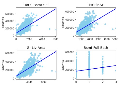
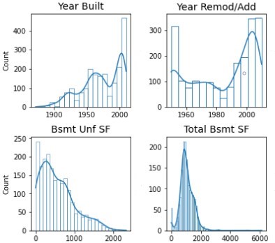
- Secondly, there must be multivariate normality, as multiple regression assumes that the residuals are normally distributed. Most of our variables are normally distributed. However, there are a number of variables that are highly skewed and have multimodal distributions. We can deal with this by not using these variables or by transforming them accordingly. For variables with right-skewed distribution, you can either opt for a log transformation or a Box Cox transformation which is a bit more flexible and able to bring your variable as close as possible to a normal distribution. You can also transform your target variable which may improve your training and validation scores. Personally I found that transforming
Sale Pricedidn't help much and led to lower RMSE scores on Kaggle. I believe this is likely due to various outliers within the test data itself.
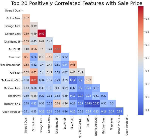
- Thirdly, there must not be multicollinearity. Multiple regression assumes that the independent variables are not highly correlated with each other. Let's do a quick check of this now. Unfortunately, according to the heatmap below, it seems that a number of features are multicollinear, with a high coefficient magnitude of >0.8. This isn't ideal, as multicollinearity will lower the precision of our estimate coefficients.
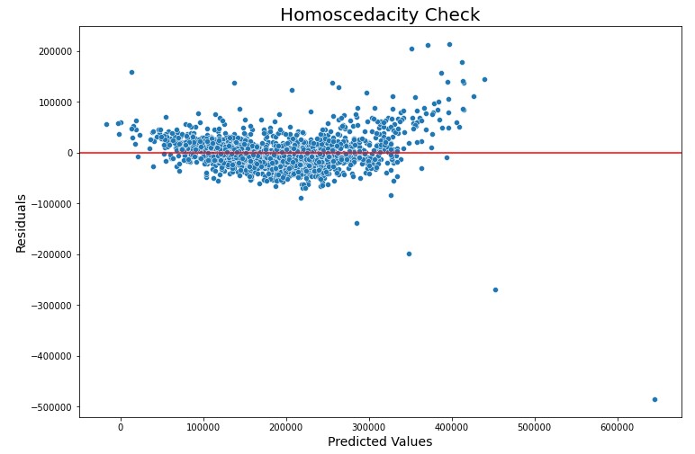
- Lastly, our independent variables must be homoscedastic. This means that the variance of error terms must be similar across the values of the independent variables. According to our scatterplot below, points are mostly equally distributed across all values of the independent variables. There also doesn't seem to be a clear pattern in the distribution. We can therefore conclude that the Ames housing data is homoscedastic.
Though using linear regression is feasible, we'll need to work to reduce multicollinearity and deal with highly skewed features further on. By performing data cleaning, feature engineering/selection and regularization, we should be able to create a linear model that can accurately predict the sale price of houses in Ames.
Data Cleaning
According to the creator of the original dataset, the entire dataset essentially takes the form of a 'data dump' from the Assessor's Office in Ames. We can expect that quite a lot of data cleaning will still need to be done.
Some of the changes that I made included:
- Removal of two
SalePricevsGr Liv Areaoutliers. There was another outlier withinGarage Yr Bltthat was an obvious error, but besides that I took a slightly more restrained approach -- removing all outliers might lead to a better score, but I felt that doing so would a bit away from the real-life challenge of predicting housing prices. In reality, there will always be outliers in terms of housing prices or certain predictors like living area. - Encoding of ordinal and categorical variables as integers. In certain cases, I chose not to adopt a conventional {0, 1, 2} order, as some variables have most houses in a single category, which then makes that the 'average' category. For example, take the
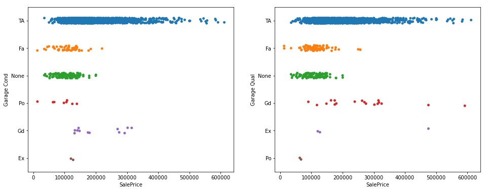
GarageQualandGarageCondfeatures. Given that the majority of houses fall into the average (TA) category for these features, it's better to set that category as 0. We'll also look to give houses with fair and no garages the similar rating, given that they have a similar range & median. My weightage of features ended up looking something like this:{'Ex':2,'Gd':1,'TA':0,'None':-0.5,'Fa':-0.5,'Po':-1}. Following this convention significantly improved the accuracy of my model.
- One-hot encoding of nominal variables. In short, I encoded features as a series of binary variables (1 or 0) representing whether a category was present or not for a particular home.
- Imputation of null & missing values. Some imputations were pretty easy to carry out. For example, houses with no pool had null values for
PoolAreaand were imputed easily as 0. Others likeLot Frontagewere slightly more complex -- while it would have been easy to just impute missing values as the mean of the lot frontage of all houses, I opted to impute lot frontage based on the average of houses in the neighborhood or specific township or section and added in a bit of randomness to prevent underestimation of variance.
def lot_frontage_gen(row):
    if np.isnan(row['Lot Frontage']):
        neighborhood = row['Neighborhood']
        nbrhd_std = df[df['Neighborhood'] == neighborhood]['Lot Frontage'].std()
        lot_frontage_mean = df[df['Neighborhood'] == neighborhood]['Lot Frontage'].mean()

        try:
            # Add in slight randomness to prevent understimation of variance
            row['Lot Frontage'] = lot_frontage_mean + np.random.randint(-nbrhd_std, nbrhd_std) / 1.25

        # If neighborhood is NAN
        except:
            pid = str(row['PID'])
            print(pid, '-- Neighborhood N/A -- imputing township average')
            sliced_pid = pid[0:3]
            lot_frontage_mean = df[df['PID'].astype(str).str.contains(sliced_pid)]['Lot Frontage'].mean()
            row['Lot Frontage'] = lot_frontage_mean

    return row
Feature Engineering & Selection
After data cleaning, we essentially moved from 81 variables to 228 variables, which greatly increased the dimensionality of our data (almost 3 times the amount of our original features!). On the surface, this might seem to be a good thing -- more features equates to more accuracy right? Unfortunately, this was not the case. When testing my data with all these features, my test RMSE was extremely high, even after regularization.
In general, adding additional features that are truly associated with our target will improve the model by leading to a decrease in test set error. However, adding noise features that are not truly associated with our target will lead to a deterioration in the model, and consequently cause increased test set error. This is because noise features increase the risk of overfitting as these features may be assigned nonzero coefficients due to chance associations with the target variable.
Additionally, while some of our new features may be relevant, the variance incurred in fitting their coefficients may outweigh the reduction in bias that they bring.
It's extremely important that each step here is undertaken with reference to a benchmark model -- depending on the steps taken so far, you need to know whether each step is actually minimizing or maximizing your loss function.
Dealing with High Pairwise Correlation
In general, high correlation between two variables means they have similar trends and are likely to carry similar information. Having a perfect pairwise correlation between two variables means that one of the variables is redundant and is generating additional noise in our data that we don't want.
Below, I created a table of variables sorted by their level of pairwise correlation to each other. In cases where features provided identical information, I dropped one of the variables. In other cases, I selected the variable that had a better correlation to SalePrice. This also informed my feature engineering efforts, where I attempted to combine features to prevent the loss of information. This type of feature is known as an interaction feature, because it represents the interaction effect between two variables. If two variables have a positively correlated effect on sale price, the product of the two features could add considerable predictive value.
I took a somewhat cautious approach here, and avoided dropping major features such as Garage Cars / Fireplaces.
# Create matrix of all feature correlations
corr_matrix = housing.corr().abs()

sol = (corr_matrix.where(np.triu(np.ones(corr_matrix.shape), k=1)
                  .astype(np.bool))
                  .stack()
                  .sort_values(ascending=False))

# Convert to dataframe and reset multi-level index
corr_df = pd.DataFrame(sol.head(20)).reset_index()

# Rename columns
corr_df.columns = 'v1', 'v2', 'pair_corr'
def corr_target(row):
    row['v1_y_corr'] = housing.corr()['SalePrice'][row['v1']]
    row['v2_y_corr'] = housing.corr()['SalePrice'][row['v2']]
    return row
# Create df with pairwise correlation and correlation to target
# If the feature isn't relatively important, the feature with lower absolute correlation to target is dropped
corr_df = corr_df.apply(corr_target, axis=1)
corr_df.head(20)
In general, I chose to drop the MS SubClass category when given a choice due to it's weaker correlation with Sale Price. It seems to be a mixture of HouseStyle, Bldg Type and Year Built, which explains the high pairwise correlation. There are also multiple errorneous classifications within this category which made me generally prefer either HouseStyle or Bldg Type as predictor variables.
# Stanardize column names
housing = housing.rename(columns={'Exterior 2nd_Wd Shng': 'Exterior 2nd_WdShing'})
housing = housing.rename(columns={'Exterior 2nd_Brk Cmn': 'Exterior 2nd_BrkComm'})
housing = housing.rename(columns={'Exterior 2nd_CmentBd': 'Exterior 2nd_CemntBd'})

ext_feats = housing.columns[housing.columns.str.contains('Exterior 1st')]

# Create interaction columns for Exterior features
for i in ext_feats:
    ext_type = i.split('_')[1]
    housing[f'Ext{ext_type}'] = housing[f'Exterior 1st_{ext_type}'] * housing[f'Exterior 2nd_{ext_type}']
    housing = housing.drop([f'Exterior 1st_{ext_type}', f'Exterior 2nd_{ext_type}'], axis=1)

# Dropping due to perfect pairwise correlation score of 1
housing = housing.drop(['Street_Grvl', 'MS SubClass_190', 'Central Air_N'], axis=1)

# Dropping due to perfect pairwise correlation with Bldg Type_Duplex
housing = housing.drop(['MS SubClass_90'], axis=1)

# Dropping ID -- Yr Sold has a higher absolute correlation to sale price
housing = housing.drop(['Id'], axis=1)

# Drop MS SubClass_80 -- same as House Style_SLevel but lower
housing = housing.drop('MS SubClass_80', axis=1)

# Drop MS SubClass_50 -- same as House Style_1.5Fin but lower
housing = housing.drop('MS SubClass_50', axis=1)

# Drop MS SubClass_45 -- same as House Style_1.5Unf but lower
housing = housing.drop('MS SubClass_45', axis=1)

# This was the only polynomial feature that helped with model accuracy out of the various others I tried
housing['Garage QualCond'] = housing['Garage Qual'] * housing['Garage Cond']
housing = housing.drop(['Garage Qual', 'Garage Cond'], axis=1)
Dealing with Low Variance
We observed earlier that many of our features have the same value. In other words, these features are approximately constant and will not improve the performance of the model. This also applies if only a handful of observations differ from a constant value. Variables with close to zero variance also violate the multivariate normality assumption of multiple linear regression.
After several rounds of trial and error, dropping 57 variables with the lowest variation seemed to return the results. Using the inbuilt .var() function from pandas, I sorted and dropped variables with a variation of less than 0.009. I also tried combining features with low variation in order to increase the chances that these features are statistically significant. There's no magical cutoff point here, but any predictor that consists of almost 100% of the same value won't be much help
low_var_list = housing.var().sort_values(ascending=True)
low_var_list = low_var_list[low_var_list.values < 0.009]
# Combining categories with small sale type numbers to make them stastically significant
housing['Combined Sale Type_Con'] = housing['Sale Type_ConLw'] + housing['Sale Type_ConLI'] \
+ housing['Sale Type_Con'] + housing['Sale Type_ConLD']
# Combining categories with low variation to try to make them stastically significant
housing['Foundation_Other'] = housing['Foundation_Slab'] + housing['Foundation_Stone'] + housing['Foundation_Wood']
low_var_drop_list = [item for item in low_var_list.index]
print(low_var_list.head(10))
housing = housing.drop(low_var_drop_list, axis=1)
Recursive Feature Elimination
We're down to 149 features, but that's still a bit too much. One method of trimming down our features further is recursive feature elimination (RFE), a feature selection method that fits a model and removes the weakest feature (or features) until the specified number of features is reached. In this particular instance, we're training the algorithm on our data and letting it rank features by their coefficient attribute. (Here, I'm referring to the coefficients obtained after fitting our model on the dataset, not a feature's Pearson correlation to SalePrice). The least important coefficient is eliminated from the list of features and the model is rebuilt using the remaining set of features. This continues until the algorithm hits the number of features selected.
After some experimentation, I found that cutting about ~28 variables helped to improve model accuracy.
features = [col for col in housing._get_numeric_data().columns if col !='SalePrice']
features
X = housing[features]
y = housing['SalePrice']
model = LinearRegression()
rfe = RFE(model, n_features_to_select=120)
rfe_fit = rfe.fit(X, y)
# Creating a dataframe to help us track how our RFE model ranks each feature
rfe_df = pd.DataFrame(columns=['Feature', 'Ranking'])
rfe_df['Feature'] = X.columns
rfe_df['Ranking'] = rfe_fit.ranking_
rfe_df.sort_values(by='Ranking', ascending=False).head(10)
rfe_drop_list = X.columns[~rfe_fit.get_support()]
rfe_drop_list
In general, I largely agree with the feature ranking above. Most of the features listed are features with either low variance or a poor correlation with SalePrice. In other cases, these features are made by redundant by another feature (e.g. Garage Area as an inferior feature compared to Garage Cars).
While some features like Year Built may seem important, in reality it's not a good predictor of SalePrice, given that the variable isn't normally distributed, and is highly left-skewed. Lot Frontage and Lot Area seem to have a somewhat ambiguous relationship with SalePrice due to various outliers that create a poor goodness-of-fit.
# Dropping features ranked as unimportant by RFE
housing = housing.drop(rfe_drop_list, axis=1)
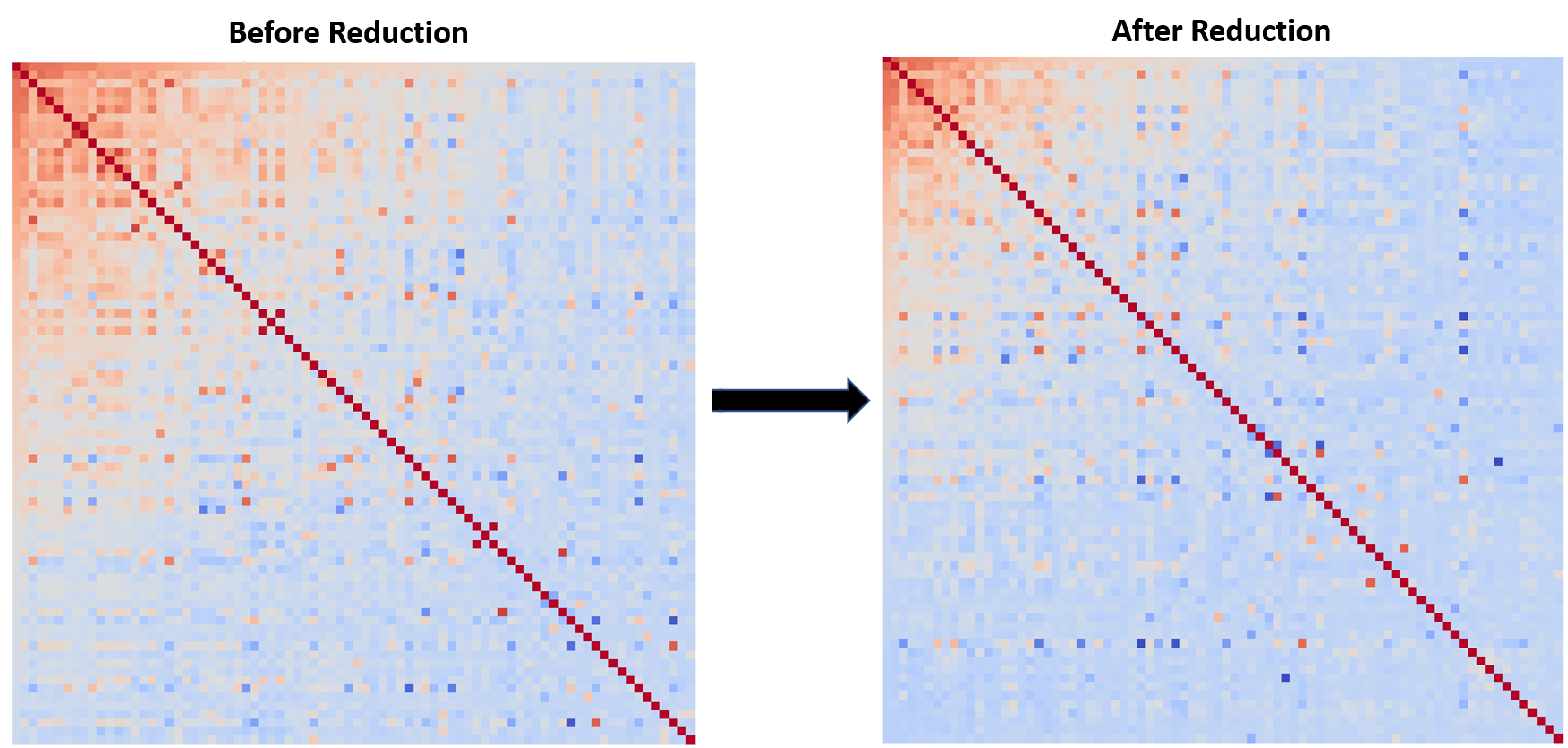
Through our efforts, we can see that multicollinearity has been reduced overall. To illustrate this, I created two heatmaps of the top 80 features correlated with SalePrice, before and after dimensionality reduction.
For the large part, it appears that there's now a lot less multicollinearity among our variables. However, a group of highly multi-correlated features remains in the top left of the heatmap below -- these are features that were too important to drop such as Gr Liv Area or Overall Qual.
Model Selection
Train Test Split & Scaling
We're standardizing our data to avoid penalizing our features simply because of their scale. This will also help us avoid avoids penalizing the intercept, which wouldn't make intuitive sense.
features = [col for col in housing._get_numeric_data().columns if col !='SalePrice']
features
X = housing[features]
y = housing['SalePrice']

X_train, X_test, y_train, y_test = train_test_split(X, y, test_size=0.3, random_state=42)

ss = StandardScaler()
ss.fit(X_train)

X_train_scaled = ss.transform(X_train)
X_test_scaled = ss.transform(X_test)
Instantiate Models
Given that there's still multicollinearity in our data, we're also going to try out a few different types of regluarization alongside a standard linear regression model.
lr = LinearRegression()
ridge = RidgeCV(alphas=np.linspace(1, 200, 100))
lasso = LassoCV(n_alphas=100)
enet_alphas = np.arange(0.5, 1.0, 0.005)
enet_ratio = 0.5
enet = ElasticNetCV(alphas=enet_alphas, l1_ratio=enet_ratio, cv=5)
Observing the Effects of Regularization
Without any form of regularization, we see that certain coefficients leading to massive skyrocketing predictions that can cause up to a roughly 120,700,700 dollar increase in predicted sale price. Running a linear regression model with large coefficients and no regularization might even result in a negative R2 accuracy. No bueno.
As a quick recap, regularization is a method for "constraining" or "regularizing" the size of the coefficients, thus "shrinking" them towards zero. It reduces model variance and thus minimizes overfitting. If the model is too complex, it tends to reduce variance more than it increases bias, resulting in a model that is more likely to generalize.
# Plotting the effects of different regularization on our linear regression model vs vanilla linear regression
fig, ax = plt.subplots(1,2, figsize=(16,6))
ax = ax.ravel()
g = sns.lineplot(data=lasso.coef_, ax=ax[0])
sns.lineplot(data=ridge.coef_, ax=ax[0], color='orange')
sns.lineplot(data=enet.coef_, ax=ax[0],color='skyblue')
g.set_xlabel('Features', fontsize=14)
g.set_ylabel('Coefficients', fontsize=14)
g.legend(title='Models', loc='upper right', labels=['Lasso', 'Ridge', 'ElasticNet'])

g2 = sns.lineplot(data=lr.coef_, ax=ax[1], color='red')
g2.legend(title='Models', loc='upper right', labels=['Linear'])

plt.tight_layout()
plt.suptitle('Regularization versus Standard Linear Regression', fontsize=22, y=1.05)

Conclusion & Recommendations
Based on the scores returned from Kaggle, our Lasso model was the most successful in predicting housing sale prices. On the dataset comprising of 30% of the test data, the model achieved an RMSE of 26658. On the dataset comprising of the other 70% of the test data, the model performed within expectations, returning an RMSE of 29400. This is a strong improvement over the baseline RMSE (~80,000) generated by using the mean of all sale prices as predictions. This answers our problem statement of how we can best predict housing prices.
Earlier versions of the model without systematic feature engineering saw up to a difference of 9,000 in terms of RMSE when given the two different test datasets. Overall, the model seems to have become much more generalizable and consistent. It also has a high R2 on our training data, where it can explain up to 91.5% of the variance in sale price.
# Fit LassoCV model to data
lasso.fit(X_train_scaled,y_train)
ridge.fit(X_train_scaled,y_train)
enet.fit(X_train_scaled,y_train)
lr.fit(X_train_scaled,y_train)
# Create scatterplot to show predicted values versus actual values
lasso_preds = lasso.predict(X_test_scaled)

plt.figure(figsize=(10,8))
sns.regplot(data=X_train_scaled, x=lasso_preds, y=y_test, marker='x', color='skyblue', line_kws={'color':'black'})
plt.xlabel('Predicted Sale Price', fontsize=14)
plt.ylabel('Actual Sale Price', fontsize=14)
plt.title('Lasso Predictions of Sale Price vs Actual Sale Price', fontsize=22)

I'm pretty happy with how the model performed in terms of predicted price versus actual price. We can see that the line of best fit passes through most of the points, barring a couple of outliers in the extreme sale price range.
ax = sns.scatterplot(data=housing, x=y_test, y=y_test-lasso_preds)
ax.axhline(y=0, c='red')
plt.xlabel('Predicted Sale Price', fontsize=12)
plt.ylabel('Actual Sale Price', fontsize=12)
plt.title('Residuals', fontsize=18)

Our residuals also mostly equally distributed, which supports the multiple linear regression assumption of homoscedasticity, i.e. variance of error terms must be similar across the values of the independent variables.
# Create dataframe of features, coefficients and absolute coefficients
lasso_df = pd.DataFrame(columns=['Feature', 'Coef', 'Abs Coef'])
lasso_df['Abs Coef'] = abs(lasso.coef_)
lasso_df['Coef'] = lasso.coef_
lasso_df['Feature'] = features

# Plot top 30 features (sorted by absolute regression coefficient)
plt.figure(figsize=(12,10))
data = lasso_df.sort_values(by='Abs Coef', ascending=False).head(30)[['Feature', 'Coef']] \
               .sort_values(by='Coef', ascending=False).reset_index(drop=True)

ax = sns.barplot(data=data, y='Feature', x='Coef', orient='h', palette='Spectral')
ax.set_ylabel('')
ax.set_yticklabels(data['Feature'], size=11)
ax.set_xlabel('Lasso Regression Coefficient', fontsize=14)
plt.title('Top 30 Housing Features', fontsize=20);

The top predictive features for our model seem pretty plausible. Our top features are living area and overall quality, followed by a range of features looking at basement square footage and the quality of the exterior and kitchen. Home functionality and the number of cars that a garage can fit are also important in predicting sale price. Certain neighborhoods like Northridge Heights and Stone Brook also are strong positive predictors.
Conversely, we see that houses that are in MS SubClass_120 (1 story houses built in 1946 and after, as part of a planned unit development) predict lower prices. The Old Town neighborhood also predicts lower prices, along with certain features such as the number of kitchens or bedrooms above ground. Having two stories also hurts the value of the home.
Understanding feature coefficients
As I mentioned previously, feature coefficients can be interpreted as β1 in the following linear regression equation:
$$ Y = \beta_0 + \beta_1 X_1 + \varepsilon$$
Here, β1 represents the estimated slope parameter, which affects the predicted value of Y. In other words, for every 1 unit change in Gr Liv Area, our target variable SalePrice or Y will increase by \$27,981. This number is pretty high, which makes it easy for our model to become overfit, as even a slight increase in Gr Liv Area will lead to a much larger shift as compared to a 1 unit change for any of our other features.
Our model intercept or β0 is \$18,147, which suggests that when our predictors are equal to 0, the mean sale price is \\$18,147. This isn't of much use however, as our X will never be 0.
In short, we can interpret our Gr Liv Area coefficient's effect on our model as:
Recommendations
Based on our model, a person looking to increase the value of their house could do the following:
- Try to increase the overall and exterior quality of their home through renovation.
- Switch to a cement or brick exterior if using a hardboard or stucco exterior.
- Improve garage size to allow it to fit more than one car.
- Focus on creating a single indoor kitchen (if they has two kitchens).
- Reduce the number of bedrooms in the house, or renovate existing bedrooms to make them multi-purpose rooms (if the house has more than three bedrooms).
While this model generalizes well to the city of Ames, it's probably not generalizable to other cities, given that each city tends to differ greatly in terms of external factors like geographical features, seasonal weather or the economic climate of that particular city.
Another point to keep in mind that this model doesn't take into account the inflation of housing prices. Since the end of the financial crisis in 2008, housing prices throughout the US have been increasing steadily year over year. Our model would need significant retraining to predict the current house prices in Ames today.
Model Limitations
Tradeoffs between interpretability and accuracy
A key consideration in this project was whether to create a more interpretable model that had a total of 30 or fewer features. Ultimately, I decided against this as this led to a significant tradeoff in accuracy. Using RFE to select 30 features greatly reduced my model's R2 and RMSE -- I believe that in this case it's not worth trading off model complexity for accuracy, given the model's current performance with less than 100 features.
This however does create some limitations. For one, some of the negative predictors are hard to interpret without extensive domain knowledge. For example, on the surface, it doesn't seem logical for the number of kitchens or bedrooms to be negative predictors for price. This can be explained by the fact that these features are acting as a proxy for other features.
For Kitchen AbvGr, I realized that houses with two kitchens have a lower mean sale price and were older compared to houses with one kitchen. In Iowa, summer kitchens were used prior to electricity and air conditioning to keep the heat from cooking out of the house during hot summer months. In colder months, the indoor kitchens were used to help keep the house warm. The fact that houses with two kitchens generally don't have much porch square footage supports this idea (as summer kitchens are generally located on the back porch). This suggests that houses with two kitchens are more likely to be antiquated houses without a good heating/ventilation system.
Submission
# Refit model on entire training dataset
X_scaled = ss.fit_transform(X)
lasso = LassoCV()
lasso.fit(X_scaled, y)
lasso.score(X_scaled,y)
# Remaining features after zeroing by lasso regression
print('Total Features before Lasso regression:', len(features))
print('Features Zeroed by Lasso regression:', len(lasso.coef_[lasso.coef_ == 0]))
print('Features Remaining after Lasso regression:', len(features) - len(lasso.coef_[lasso.coef_ == 0]))
final_test_scaled = ss.transform(test)
final_predictions = lasso.predict(final_test_scaled)
test['SalePrice'] = final_predictions
test['Id'] = test_ids
# Create csv for submission
submission = test[['Id','SalePrice']]
submission.to_csv('./datasets/kaggle_submission.csv', index=False)

#View submission
submission.head()