Capstone Project: Predicting New York Times Article Popularity¶

Introduction¶

The New York Times is one of the most popular news platforms in the world and is visited by a countless number of visitors each day. The Times' focus on subscribers sets them apart in crucial ways from other media organizations. Instead of trying to maximize clicks and sell low-margin advertising, the Times believes in providing high quality journalism and building up reader loyalty through community engagement.

In 2020 alone, there were nearly 5,000,000 comments posted on New York Times articles. That's 13,000 comments per day. While the Times has adopted machine learning to improve the comment moderation process, a large part of the moderation is still done by hand. In short, the New York Times can't allow comments on every article due to manpower restraints.

This is the problem my project aims to resolve. Having the probability of whether an article is popular or unpopular can help improve the allocation of moderation resources. This will improve comment moderation efficiency, and potentially lead to a larger number of articles being opened for comments.

This could also allow the Times staff to make tweaks to increase article popularity before publishing an article, if they so desire.

This project therefore aims to answer:

How can the NYT staff improve article popularity?
Can we accurately predict article popularity? What are the most important predictors?

Executive Summary¶

For this project, I scraped over 16,000 articles and 5,000,000 comments from January - December 2020 using the nyt-scraper package.

The top-performing model was a XGBoost Classifier which achieved an ROC-AUC score of 0.869 and an accuracy of 0.786. A wide range of feature engineering techniques were used to accomplish this, including sentiment analysis and transformation of categorical features to ordinal features based on overall average popularity.

Generally, I found that an article's news desk, section, and subsection had a heavy influence on whether it was popular or not. Text-based features like overall word count, headline/abstract length also played a key role. Longer articles tended to be more popular, while having a shorter headline/abstract generally improved popularity.

The sentiment of the headline/abstract also affected popularity, where articles with a more negative headline/abstract did better than articles with a neutral headline/abstract. The hour of publication also had an effect on popularity, where articles published late at night tended to draw more comments.

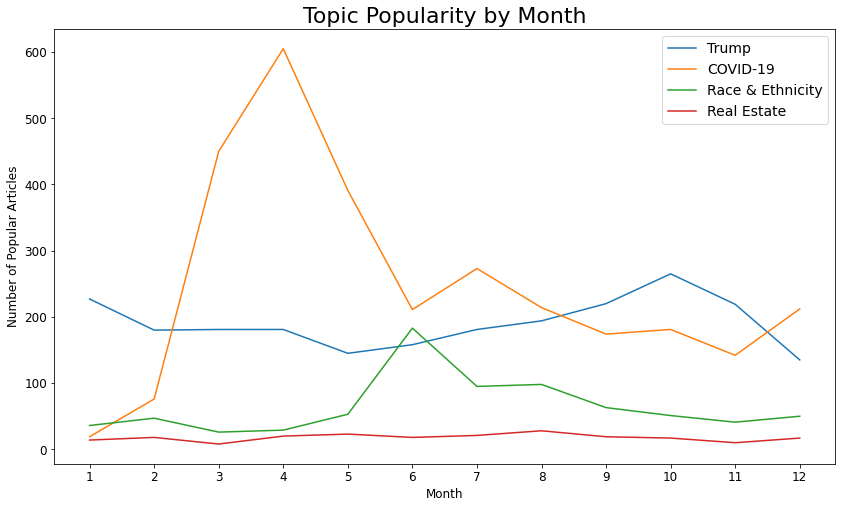
Additionally, certain topics tended to be naturally more popular. Around 80% of articles mentioning Donald Trump each month had more than 90 comments, while only 20% or 30% articles around Real Estate news drew more than 90 comments.

The full code for this project is available on Github.

Data Scraping¶

I chose to scrape data from the New York Times as they are one of the very few media publications that offer a wide range of APIs that are open to the public.

The New York Times currently offers 10 public APIs: Archive, Article Search, Books, Community, Geographic, Most Popular, Semantic, Times Newswire, TimesTags, and Top Stories.

To scrape articles from the NYT, you need to sign up for a free developer’s account which will give you an API key you can use to get article and comment meta data. A detailed guide for the sign-up process can be found here.

Instead of manually scraping the data by hand, I opted to use the nytimes-scraper package on Github for this, which allowed me to scrape over 16,000 articles and around 5,000,000 comments from January 2020 to December 2020.

The documentation for the NYT articles / comments APIs can be found here and here.

# This is the code that I used to scrape NYT articles from Jan - Dec
import datetime as dt
from nytimes_scraper import run_scraper, scrape_month

article_df, comment_df = scrape_month('<API KEY>', date=dt.date(2020, 1, 1))

Data Cleaning & Preprocessing¶

After scraping the files from the NYT articles and comments API, I was left with pickle files for every comment and article for each month. Together, the size of the article files were about 19GB, while the comment pickle files were about 3GB. This was initially an issue as it was slightly too big to process with, so I experimented with Dask and SQL before ultimately I settled on reducing the size of my datasets by dropping unnecessary columns and text.

I had several objectives during this data cleaning process:

Calculate number of comments for each article by joining each comment and article file on ArticleID.
Create a classification category is_popular by sorting comments above and below a certain number.
Create a train and test dataset for classification.
Reduce file size by dropping unnecessary columns.
Avoid copyright issues by dropping article text and only keeping the headline and abstract.

The full data cleaning process can be viewed here.

Summary of Changes¶

Comments:

Dropped status, commentTitle, userURL, picURL, userLocation, userDisplayName, trusted, isAnonymous, updateDate permID and parentUserDisplayName to slightly reduce file size and avoid the risk of accidentally doxxing NYT commenters.

Articles:

Dropped print_section & print_page as we are only concerned with online articles.
Dropped most headline.* features as they contain a large number of null values, which make them unuseful as predictors for modelling.
Dropped text & html to avoid copyright issues.
Dropped uri as it seems to be the same as article ID
Dropped byline.organization as it has a high amount of null values.
Dropped byline.person as byline.original is more informative
Changed keywords data structure from nested dictionary to list of keywords per article
Renamed and re-organized columns to make them a bit more user-friendly.

Exploratory Data Analysis¶

Popularity vs Number of Comments¶

There's a large group of articles that have less than 90 comments -- this is where I chose to split the data. We can see that n_comments has a heavy positive skew, with the number of articles decreasing in proportion to the number of comments.

It's important to note here that not all NYT articles are open for comments. The NYT moderation team chooses articles to open for public commentary. Our data only reflects articles that were opened for commentary AND recieved at least one comment.

# Average number of comments
train['n_comments'].mean()

305.8529549718574

fig, ax = plt.subplots(1,1, figsize=(16,8))
sns.histplot(train['n_comments'].drop(train[train['n_comments'] > 3000].index), bins=35)
mean = train['n_comments'].mean()
plt.axvline(90, ls='-', c='red', label='Split', lw=4)
plt.legend(fontsize=12, loc=1)
plt.xlabel('Number of Comments')
plt.ylabel('Number of Articles')
plt.title(f'Number of Comments', fontsize=18)

Text(0.5, 1.0, 'Number of Comments')

Checking Class Balance¶

plt.figure(figsize=(10,6))
with warnings.catch_warnings():
    warnings.simplefilter("ignore")
    
    # Overall, our classes are pretty much evenly balanced
    g = sns.countplot(train['is_popular'])
    g.set_xticklabels(['Unpopular (< 90 comments)', 'Popular (> 90 comments)'])
    plt.xlabel('')
    plt.ylabel('Number of Articles')
    plt.title('Class Balance', fontsize=16);

# Our positive class is only slightly smaller than our negative class
train['is_popular'].value_counts(normalize=True)

0    0.503752
1    0.496248
Name: is_popular, dtype: float64

# There are a few extreme outliers in our data
plt.figure(figsize=(16,4))
sns.boxplot(data=train['n_comments'], orient='h')
plt.xlabel('n_comments')
plt.yticks([])
plt.xlabel('Number of Comments')
plt.title('Number of Comments', fontsize=18);

# Top 3 outliers
train[train['n_comments'] > 4000][['headline', 'abstract', 'n_comments', 'pub_date']] \
.sort_values(by='n_comments', ascending=False).head(3)

Word Count¶

Dealing with word count is slightly tricky. We can see that the feature is normally distributed in general with a heavy positive skew. We can also see that there are a large number of articles that have a word count of 0. These are interactive features that don't have 'words' in the conventional sense. Because this is not technically 'missing' data, I'm not going to impute it.

# Close to a normal distribution, with a positive skew
plt.figure(figsize=(16,8))
mean = train['word_count'].mean()
plt.axvline(mean, ls='--', color='black')
sns.histplot(train['word_count'])
plt.xlabel('Word Count')
plt.title(f'Word Count (Mean: {mean:.0f} words)', fontsize=18);

In general, machine learning algorithms tend to perform better when the distribution of variables is normal -- in other words, performance tends to improve for variables that have a standard distribution.

Feature Transformation¶

def transform_var(col, df):
    skew_dict = {} # Creating dictionary to store skew values
    df[f'{col}_log'] = np.log1p(df[f'{col}'])
    df[f'{col}_box'] = df[f'{col}'].replace(0, 0.001) # Replacing as Boxcox can't transform values that are 0
    df[f'{col}_box'] = boxcox(df[f'{col}_box'])[0]
    df[f'{col}_sqrt'] = np.sqrt(df[f'{col}'])
    
    skew_dict['Original'] = df[f'{col}'].skew()
    skew_dict['Log1p'] = df[f'{col}_log'].skew()
    skew_dict['Boxcox'] = df[f'{col}_box'].skew()
    skew_dict['Square Root'] = df[f'{col}_sqrt'].skew()
    return skew_dict

def plot_transform(col, df):
    fig, ax = plt.subplots(2, 2, figsize=(13,9), sharey=True)
    ax = ax.ravel()
    sns.histplot(df[f'{col}'], ax=ax[0])
    ax[0].set_title(f"Original (Skew: {skew_dict['Original']:.3f})", fontsize=14)
    sns.histplot(df[f'{col}_log'], ax=ax[1])
    ax[1].set_title(f"Log1p (Skew: {skew_dict['Log1p']:.3f})", fontsize=14)
    sns.histplot(df[f'{col}_box'], ax=ax[2])
    ax[2].set_title(f"Boxcox (Skew: {skew_dict['Boxcox']:.3f})", fontsize=14)
    sns.histplot(df[f'{col}_sqrt'], ax=ax[3])
    ax[3].set_title(f"Square Root (Skew: {skew_dict['Square Root']:.3f})", fontsize=14)
    for ax in ax:
        ax.set_xlabel('')
        ax.set_ylabel('')
    plt.suptitle('Transformed Word Count', fontsize=18)
    plt.tight_layout()

Here, we can see the effectiveness of various transformation methods. The Boxcox transformation seems to work best here -- our data is still slightly skewed but much closer to a normal distribution.

skew_dict = transform_var('word_count', train)
plot_transform('word_count', train)

# There are a few extreme outliers in our data
plt.figure(figsize=(16,4))
sns.boxplot(data=train['word_count'], orient='h')
plt.yticks([])
plt.xlabel('Word Count')
plt.title('Word Count', fontsize=18);

Number of Comments versus Word Count¶

Does word count, or the length of an article affect the number of comments on each article? In the plot below, we can see that there's generally a positive relationship between these two variables, except for OpEd articles where it seems that word count doesn't affect number of comments at all. OpEd articles have an average of around 1100 words.

# Combining different newsdesk names
plt.figure(figsize=(12, 10))
train['newsdesk'] = train['newsdesk'].apply(lambda x: 'The Upshot' if x=='Upshot' else x)
train['newsdesk'] = train['newsdesk'].apply(lambda x: 'OpEd' if x=='Opinion' else x)
train['newsdesk'] = train['newsdesk'].apply(lambda x: 'AtHome' if x=='At Home' else x)

# OpEd length doesn't affect number of comments -- but longer news from the Washington desk does
g = sns.lmplot(data=train.loc[train['newsdesk'].isin(top_news_df)], x='word_count', y='n_comments', 
               hue='newsdesk', palette='tab10', height=8, aspect=1.10, scatter_kws={'alpha':0.3, 's':15}, legend_out=False)

for lh in g._legend.legendHandles: 
    lh.set_alpha(1)
    lh._sizes = [20] 

g._legend.set_title('News Desk')

plt.ylabel('Number of Comments', fontsize=11)
plt.xlabel('Word Count', fontsize=11)
plt.legend(fontsize=14)
plt.title('Number of Comments versus Word Count', fontsize=18);

# There's a moderate positive correlation between these two variables
train.corr()['is_popular']['word_count']

0.1713162393600203

News Desk¶

These are the newsdesks with the most number of comments. Unsurprisingly, OpEd articles are at the top, followed by Foreign and Business. In 2017, the NYT implemented a new commenting system that opened up OpEd articles and other selected news articles for 24 hours. This is likely part of the reason why OpEd articles seem to draw a higher frequency of comments.

# Grouping largest 20 newsdesks and sorting by popularity
df = train['newsdesk'].value_counts(ascending=False).reset_index()
df.columns=['newsdesk', 'n_articles']
temp = pd.merge(df, train.groupby('newsdesk').mean()['is_popular'].reset_index()).head(10)
temp['n_articles'].sum()

7364

g_index = df['newsdesk'].head(20).values
g_df = train[train['newsdesk'].isin(g_index)]
g_data = g_df.groupby('newsdesk').mean()['is_popular'].sort_values(ascending=False)
g_data = g_data.to_frame().reset_index()
g_data.head()

# Top 20 newsdesks
plt.figure(figsize=(12, 10))
sns.barplot(data=g_data, y=g_data['newsdesk'], x=g_data['is_popular'], orient='h', palette='coolwarm_r')
plt.xlabel('Average Popularity')
plt.ylabel('Newsdesk')
plt.xticks(np.arange(0.0, 1.1, 0.1), fontsize=12)
plt.yticks(fontsize=12)
plt.title('Newsdesk Avg. Popularity', fontsize=18);
plt.axvline(0.5, ls='--', color='black');

Feature Engineering¶

Word Count¶

We saw previously that the Boxcox transformation seems to work best, so we'll use that going forward. We'll also keep the original word count variable as removing it led to a drop in model accuracy.

section_avg = train.groupby('section').mean()['word_count']

train['boxcox_word'] = train['word_count'].apply(lambda x: 0.001 if x == 0 else x)
train['boxcox_word'] = boxcox(train['boxcox_word'])[0]

Time Variables¶

Time affects the frequency of published articles, which correspondingly affects the popularity of articles. Articles published at a time where less articles are published are more likely to be more popular -- there's less places for commentators to go.

train['day_of_month'] = train['pub_date'].apply(lambda x: x.day)
train['day_of_week'] = train['pub_date'].apply(lambda x: x.dayofweek)
train['hour'] = train['pub_date'].apply(lambda x: x.hour)
train['is_weekend'] = train['day_of_week'].apply(lambda x: 1 if x==5 or x==6 else 0)

I also created an additional variable that tracks when an article was published. Articles published between 10PM and 2AM seem to have to have a much higher average popularity.

train['is_primehour'] = train['hour'].apply(lambda x: 1 if x > 22 else 1 if x < 4 else 0)

train.corr()['is_popular']['is_primehour']

0.16983850369317796

Articles Per Day¶

Similar to our time variables, I created a variable that tracks the number of articles posted in a day. The idea is that the less articles there are, the higher the popularity and vice versa.

train['group_date'] = train['pub_date'].astype(str).apply(lambda x: x[:10])
group_dates = train['group_date'].value_counts()
train['posts_per_day'] = train['group_date'].apply(lambda x: group_dates[x])

# More posts in a day correlated with lower popularity
train.corr()['is_popular'][['posts_per_day']]

posts_per_day   -0.1039
Name: is_popular, dtype: float64

Keywords¶

Having a certain number of keywords seems important -- the ideal number of keywords seems to be between 11 and 16. This could suggest that people are more interested in articles that cover a range of topics, people and organizations.

train['n_keywords'] = train['keywords'].apply(lambda x: len(x))
train['ideal_n_keywords'] = train['n_keywords'].apply(lambda x: 1 if x == 1 else 1 if (x > 11 and x < 16) else 0)

train.corr()['is_popular'][['n_keywords', 'ideal_n_keywords']]

n_keywords          0.072866
ideal_n_keywords    0.143074
Name: is_popular, dtype: float64

Trump / Republican / Democrat¶

We saw that Donald Trump and Republican/Democrat keywords are among the most frequent keywords, so we'll create a variable here to keep track of that. Both these features have a significant correlation with popularity.

train['is_trump'] = train['keywords'].apply(lambda x: 1 if 'Trump, Donald J' in x else 0)

train['is_party'] = train['keywords'].apply(lambda x: 1 if 'Democratic Party' in x 
                                                else 1 if 'Republican Party' in x else 0)

train.corr()['is_popular'][['is_trump', 'is_party']]

is_trump    0.273985
is_party    0.201494
Name: is_popular, dtype: float64

Race & Ethnicity¶

Race and ethnicity has always been a hot topic in the US, and especially so this year with the death of George Floyd. This has a slight correlation with article popularity.

train['is_racial'] = train['keywords'].apply(lambda x: 1 if 'Black People' in x 
                                                else 1 if 'Race and Ethnicity' in x 
                                                else 1 if 'Discrimination' in x
                                                else 1 if 'Black Lives Matter Movement' in x
                                                else 0)

train.corr()['is_popular'][['is_racial']]

is_racial    0.062983
Name: is_popular, dtype: float64

COVID-19¶

COVID-19 has drastically changed the world as we know it -- it was also the most frequent keyword in our entire dataset. All three features below have a faint correlation with popularity.

train['is_covid'] = train['keywords'].apply(lambda x: 1 if 'Coronavirus (2019-nCoV)' in x \
                                                else 1 if 'Coronavirus Risks and Safety Concerns' in x 
                                                else 0)

train['is_epidemic'] = train['keywords'].apply(lambda x:1 if 'Epidemics' in x else 0)

train['is_death'] = train['keywords'].apply(lambda x: 1 if 'Deaths (Fatalities)' in x else 0)

train.corr()['is_popular'][['is_covid', 'is_epidemic', 'is_death']]

is_covid       0.071195
is_epidemic    0.069257
is_death       0.046664
Name: is_popular, dtype: float64

Question¶

If the headline or abstract contains a question mark, there's a good chance that the article has been written in a way to invite commentary. Alternatively, people might view the question mark as a friendly invitation to comment.

train['headline_question'] = train['headline'].apply(lambda x: 1 if '?' in x else 0)

train[train['headline_question'] == 1]['is_popular'].value_counts()

1    954
0    685
Name: is_popular, dtype: int64

train['abs_question'] = train['abstract'].apply(lambda x: 1 if '?' in x else 0)

train[train['abs_question'] == 1]['is_popular'].value_counts()

1    508
0    387
Name: is_popular, dtype: int64

train.corr()['is_popular'][['headline_question', 'abs_question']]

headline_question    0.065796
abs_question         0.039141
Name: is_popular, dtype: float64

Newsdesk / Section / Subsection / Material¶

An article's newsdesk, section, subsection are likely the most powerful predictors of popularity. Opinion Editorials (OpEds) are much more likely to draw comments because they're likely written in a way to attract attention or controversy. These OpEds tackle recent events and issues, and attempt to formulate viewpoints based on an objective analysis of happenings and conflicting/contrary opinions. NYT Opinion pieces are also always open for comments, which would naturally increase the likelihood of having a popular article.

It was pretty difficult to decide on how to map / encode these features. There are 60 newsdesks, 42 sections, 67 subsections, and 10 types of material. Performing a one hot encoding on each variable would leave me with over 180 features in total.

There are several approaches that I tried:

One hot encode Newsdesk, Section and Subsection (this returned poor results)
Combine Newsdesk, Section and Subsection into a single NewsType variable
- For example: Foreign newsdesk, World section, Australia Subsection --> #Foreign#World#Australia.
- Group similar articles together e.g. #Foreign#World#Australia and #Foreign#World#Asia Pacific. This naturally presents some difficulty though -- how do we decide which sections and subsections to group together? The Australia subsection has more popular articles but only has 46 articles compared to the 327 articles in the Asia Pacific subsection.
Create an ordinal interaction feature (number of popular articles * total number of articles) that gives a higher weight to features that have many popular articles and a large number of total articles.
Use DBSCAN or other clustering methods to group variables together.

Ultimately, I found that taking a simpler approach returned better results. Below, I created a function that groups features according to their average popularity. In short, I created an ordinal feature that places more weight on newsdesks/sections/subsections/materials that have an average popularity of 0.6 and above. Conversely, I placed a low weight on variables that have a average popularity of 0.4 and below.

To catch unique newsdesks/sections/subsections/materials that are in the test but not in train dataset, I added in an if statement that maps these unique sections to 0. This should cause our model to treat them in a neutral way.

# Combining newsdesks -- the different names reflect interactive articles that will be accounted for later
train['newsdesk'] = train['newsdesk'].apply(lambda x: 'The Upshot' if x=='Upshot' else x)
train['newsdesk'] = train['newsdesk'].apply(lambda x: 'OpEd' if x=='Opinion' else x)
train['newsdesk'] = train['newsdesk'].apply(lambda x: 'AtHome' if x=='At Home' else x)

# We have to fill the null values in our subsection
train['subsection'].fillna('N/A', inplace=True)

def map_popularity(col):
    df = train.groupby(f'{col}').mean().reset_index().sort_values(by='is_popular', ascending=False) \
              [[f'{col}', 'is_popular']]
    df.columns=[f'{col}', 'avg_popularity']
    
    pop_5 = df[df['avg_popularity'] >= 0.7][f'{col}'].values
    pop_4 = df[(df['avg_popularity'] < 0.7) & (df['avg_popularity'] >= 0.6)][f'{col}'].values
    pop_3 = df[(df['avg_popularity'] < 0.6) & (df['avg_popularity'] >= 0.5)][f'{col}'].values
    pop_2 = df[(df['avg_popularity'] < 0.5) & (df['avg_popularity'] >= 0.4)][f'{col}'].values
    pop_1 = df[(df['avg_popularity'] < 0.4) & (df['avg_popularity'] >= 0.3)][f'{col}'].values
    pop_0 = df[df['avg_popularity'] < 0.3][f'{col}'].values
    
    def lambda_fxn(x):
        if x in pop_5:
            return 5
        elif x in pop_4:
            return 4
        elif x in pop_3:
            return 3
        elif x in pop_2:
            return 2
        elif x in pop_1:
            return 1
        elif x in pop_0:
            return -1
        
        # To catch news desks/sections/subsections/material in test but not in train
        else:
            return 0
    
    train[f'{col}_pop'] = train[f'{col}'].apply(lambda_fxn)
    test[f'{col}_pop'] = test[f'{col}'].apply(lambda_fxn)

map_popularity('newsdesk')

map_popularity('section')

map_popularity('subsection')

map_popularity('material')

# Example of mapping newsdesk / section / subsection / material
train.loc[101][['headline', 'newsdesk', 'newsdesk_pop', 'section', 'section_pop', 'subsection', 
                'subsection_pop', 'material', 'material_pop']].to_frame().T

Other Features¶

train['combi_text'] = train['headline'] + '. ' + train['abstract']

Sentiment¶

Sentiment plays a notable role in determining popularity. People are more likely to comment on articles with headlines that have negative sentiment, and less likely to comment on articles with headlines that have neutral sentiment. Previous research has shown that content that evokes high-arousal positive (awe) or negative (anger or anxiety) emotions tends to be more viral.

train['combi_text'][0]

'Protect Veterans From Fraud. Congress could do much more to protect Americans who have served their country from predatory for-profit colleges.'

# Instantiating sentiment intensity analyzer
sia = SIA()
sia.polarity_scores(train['combi_text'][0])

{'neg': 0.139, 'neu': 0.66, 'pos': 0.201, 'compound': 0.1725}

def get_sentiment(row):
    sentiment_dict = sia.polarity_scores(row['combi_text'])
    row['sentiment_pos'] = sentiment_dict['pos']
    row['sentiment_neu'] = sentiment_dict['neu']
    row['sentiment_neg'] = sentiment_dict['neg']
    row['sentiment_compound'] = sentiment_dict['compound']
    return row

train = train.progress_apply(get_sentiment, axis=1)

100%|███████████████████████████████████████████████████████████████████████████| 12792/12792 [00:26<00:00, 476.11it/s]

# Looks like negative articles tend to be more popular
train.corr()['is_popular'][['sentiment_compound', 'sentiment_pos', 'sentiment_neu', 'sentiment_neg']]

sentiment_compound   -0.101446
sentiment_pos        -0.009546
sentiment_neu        -0.105958
sentiment_neg         0.136188
Name: is_popular, dtype: float64

Headline / Abstract Length¶

The idea here is that longer headlines and abstracts will lead to less comments -- the easier the headline / abstract is to understand, the more comments the article will attract. We can see this seems to be a factor for the abstract, while headline length doesn't seem to have much of an impact.

train['headline_len'] = train['headline'].apply(lambda x: len(x))
train['abstract_len'] = train['abstract'].apply(lambda x: len(x))

train['head_abs_len'] = train['headline_len'] + train['abstract_len']

# Shorter abstracts seem to do better
train.corr()['is_popular'].sort_values(ascending=False)[['abstract_len', 'headline_len']]

abstract_len   -0.104951
headline_len   -0.001611
Name: is_popular, dtype: float64

Interactive Features¶

There are only a few interactive features, but generally I found that including this feature increased my model accuracy.

train['is_interactive'] = train['material'].apply(lambda x: 1 if x == 'Interactive Feature' else 0)

Clustering¶

I also tried out various clustering methods on my data to see if there was a more efficient way of clustering by newsdesk or section, or by headline. Generally, I found that clustering didn't help my model accuracy much. The headlines also seemed clustered pretty close together, which made it difficult for DBSCAN effectively separate them. Using K-means clustering seemed to work slightly better, but the topics ended up looking pretty similar. I excluded clustering from my final model, but it's worth noting that some clusters, particularly cluster 4 had a moderate correlation with popularity.

Feature Correlation with Target¶

plt.figure(figsize=(10,12))
sns.heatmap(train.corr()[['is_popular']].sort_values(ascending=False, by='is_popular'), 
            cmap='coolwarm', annot=True, vmax=0.8)

<AxesSubplot:>

Modelling¶

The top-performing model was a XGBoost Classifier which achieved an ROC-AUC score of 0.869 and an accuracy of 0.786.

Generally, I found that an article's news desk, section, and subsection had a heavy influence on whether it was popular or not. Text-based features like overall word count, headline/abstract length also played a key role. Longer articles tended to be more popular, while having a shorter headline/abstract generally improved popularity.

The sentiment of the headline/abstract also affected popularity, where articles with a more negative headline/abstract did better than articles with a neutral headline/abstract. The hour of publication also had an effect on popularity, where articles published late at night tended to draw more comments.

Additionally, certain topics tended to be naturally more popular. Around 80% of articles mentioning Donald Trump each month had more than 90 comments, while only 20% or 30% articles around Real Estate news drew more than 90 comments.

# Viewing the most important features
plt.figure(figsize=(8,12))
sns.barplot(data=total_gain, y='feature', x='total gain', orient='h', palette='Blues_r')
plt.ylabel('');
plt.xlabel('Total Gain', fontsize=12)
plt.yticks(fontsize=12)
plt.xticks(fontsize=12)
plt.title('Total Gain', fontsize=18)
plt.tight_layout()
plt.savefig(fname='total_gain', dpi=180)

Based on the graph above, these are our most important features (along with some brief thoughts):

News desk - seems to be a very strong determinant. This suggests that many commentators stick to a particular news desk.
Word count (regular) - longer articles seem to be more popular except for OpEd pieces
Section - another powerful determinant. Some niche sections might draw commentators.
Material type - interactive articles and editorial/opinion pieces tend to be more popular
Number of keywords - keywords can be understood as a proxy for number of topics. Too many topics (or too little) could make an article uninteresting for many commentators.
Hour - articles tend to do better at different times of the day.
Subsection - same as section / newsdesk.
Headline length - short headlines seem to do better than long headlines in general.
Combined headline & abstract length - ibid.
Sentiment - headline & abstracts with negative sentiment tend to draw more comments.

Recommendations¶

For articles that our model predicts to be unpopular, the following can be done, based on our above analysis:

Re-write ‘neutral’ headlines & abstracts
Shorten length of headlines & abstracts and include a question mark
Change publication time to between 10pm and 3am
Make sure the story is tied to the current socio-political context and use the right keywords
Use a recommendation system to drive traffic to from popular articles to unpopular articles

This model can also be used in tandem with the moderation team's current tools to improve overall moderation efficiency.

Limitations¶

Of course, just because an article has a low number of comments doesn't necessarily mean it's a low-performing article. The article might not appeal to regular commentators, and might do better on social media.

The NYT has to also uphold a degree of journalistic integrity -- even though using a click-bait headline might get them more comments, it’s in their own interest to remain an impartial and trusted source of news.

Additionally, this model is heavily affected by an article's news desk / section / subsection. More work should be done to ensure that an article's popularity isn't over or under predicted. Other predictors that could be looked into include topic 'freshness', where topics that are new tend to do much better than old topics (unless it's about Donald Trump which is basically an evergreen topic at this point).

Final Thoughts¶

The media industry is changing pretty rapidly -- it isn't enough to put out regular news reports anymore. People are used to getting their news from social media, be it Facebook, Twitter, Instagram or Reddit. That means that they're used to being part of an online community, where anyone can share their views, and publicly agree/disagree with each other. In short, people are increasingly going to be drawn to a news platform that allow them to be part of a community.

There's also been a turn towards reader engagement in the form of interactive articles. Many millennials / Gen Z youth have obtained a pretty high standard of digital literacy. They appreciate graphs and data that personally speaks to them, versus a static page that doesn't allow for any interaction.

As digital advertising changes in the wake of digital privacy laws and changing consumer habits, newspapers and the media industry in general must drastically overhaul their business to stay profitable. This also extends to the field of public relations, which needs to adopt new tools and methodologies to be able to tell stories that people actually want to hear. This project represents an attempt at media analytics which can help both news content providers and third party news providers (e.g. public relations firms).

	headline	abstract	n_comments	pub_date
12618	Trump’s Taxes Show Chronic Losses and Years of...	The Times obtained Donald Trump’s tax informat...	8987	2020-09-27 21:07:33+00:00
2436	Bernie Sanders Is Making a Big Mistake	It has to do with respect.	5702	2020-02-23 23:33:29+00:00
6154	Democrats, It’s Time to Consider a Plan B	Tara Reade’s allegations against Joe Biden dem...	5228	2020-05-03 19:00:07+00:00

	newsdesk	is_popular
0	OpEd	0.928663
1	Politics	0.793878
2	Games	0.782857
3	Washington	0.774510
4	National	0.710526

PREDICTING ONLINE NEWS POPULARITY

Classifying the popularity of 16,000 articles from the New York Times

Capstone Project: Predicting New York Times Article Popularity¶

Introduction¶

Executive Summary¶

Data Scraping¶

Data Cleaning & Preprocessing¶

Summary of Changes¶

Exploratory Data Analysis¶

Popularity vs Number of Comments¶

Checking Class Balance¶

Word Count¶

Feature Transformation¶

Number of Comments versus Word Count¶

News Desk¶

Feature Engineering¶

Word Count¶

Time Variables¶

Articles Per Day¶

Keywords¶

Trump / Republican / Democrat¶

Race & Ethnicity¶

COVID-19¶

Question¶

Newsdesk / Section / Subsection / Material¶

Other Features¶

Sentiment¶

Headline / Abstract Length¶

Interactive Features¶

Clustering¶

Feature Correlation with Target¶

Modelling¶

Recommendations¶

Limitations¶

Final Thoughts¶