Project 4: West Nile Virus Prediction¶

Introduction¶

The West Nile Virus (WNV) has been a serious problem for the United States since 1999. The CDC has acknowledged it as the leading cause of mosquito-borne disease in the continental United States. However, there are no vaccines to prevent or medications to treat WNV in people -- according to the CDC, 1 in 5 people who are infected develop a fever and other symptoms, while 1 out of 150 infected people develop a serious, sometimes fatal, illness.

In Illinois, West Nile virus was first identified in September 2001 when laboratory tests confirmed its presence in two dead crows found in the Chicago area. The following year, the state's first human cases and deaths from West Nile disease were recorded and all but two of the state's 102 counties eventually reported a positive human, bird, mosquito or horse. By the end of 2002, Illinois had counted more human cases (884) and deaths (64) than any other state in the United States.

Since then, Illinois and more specifically Chicago, has continued to suffer from multiple outbreaks of the West Nile Virus. From 2005 to 2016, a total of 1,371 human WNV cases were reported within Illinois. Out of these total reported cases, 906 cases (66%) were from the Chicago region (Cook and DuPage Counties).

With this in mind, our project is aimed at predicting outbreaks of the West Nile Virus. This will help the City of Chicago and Chicago Department of Public Health (CDPH) more efficiently and effectively allocate resources towards preventing transmission of this potentially deadly virus. Specifically, our model will use a combination of weather, time and location features to predict the presence of WNV within mosquito traps set up throughout Chicago.

Project Description¶

This was a group project based on a Kaggle competition that asked competitors to predict whether or not West Nile Virus was present, for a given time, location, and species. The evaluation metric for prediction accuracy was ROC AUC. The data set included 8 years: 2007 to 2014. Years 2007, 2009, 2011 and 2013 were used for training while remaining four years were included in test data.

We faced a slight challenge due to the weak correlation between our target WnvPresent and all our other features. This meant data cleaning and engineering would be vital in creating an accurate prediction. The temporal aspect of this project was another thing we had to deal with. As outbreaks take time to build up, we had to pay careful attention to separating our features by day, week and month.

The full code for this project is available here.

Data Cleaning¶

Summary of Changes¶

Weather:

Imputed missing values for daily average temperature Tavg with average of Tmax and Tmin
Calculated missing values for Cool and Warm with Tavg
Calculated missing Depart from Station 2 with 30 year normal temperature based on Station 1 readings and Station 2 Tavg.
Imputed missing values for WetBulb, PrecipTotal, StnPressure, SeaLevel, AvgSpeed using readings of Station with non-missing value.
Imputed 'T' or trace values as 0.01.
Imputed Sunrise and Sunset for Station 2 with Station 1 values
Split and recombined CodeSum to create proper spacing between different codes
Created new feature counting number of exceptional weather phenomena based on CodeSum
Created more interpretable features like rain and lowvis based on CodeSum
Changed Date from string object to datetime64
Dropped Water1, Depth, SnowFall due to high missing values (>99.5% 'M' or 0)
Transformed all features into float values
Merged Station 1 and Station 2 by averaging values of each station
Added Year, Month, Week and Day of Week features

Spray:

Dropped duplicates
Dropped missing Time values

Weather¶

Initial Analysis¶

weather.head(3)

# Checking for missing values
weather.isnull().sum()[weather.isnull().sum() > 0]

Series([], dtype: int64)

# Checking for duplicate values
weather.duplicated().sum()[weather.duplicated().sum() > 0]

array([], dtype=int64)

# Many 'M' or missing values in certain columns
weather.isin(['M']).sum()[weather.isin(['M']).sum() > 0].sort_values(ascending=False)

Water1         2944
SnowFall       1472
Depth          1472
Depart         1472
Cool             11
Heat             11
Tavg             11
SeaLevel          9
StnPressure       4
WetBulb           4
AvgSpeed          3
PrecipTotal       2
dtype: int64

# Some 'T' or trace values
weather.isin(['  T']).sum()[weather.isin(['  T']).sum() > 0]

SnowFall        12
PrecipTotal    318
dtype: int64

# Checking for zero values
weather.isin(['0.0']).sum()[weather.isin(['0.0']).sum() > 0]

SnowFall    1459
dtype: int64

# Checking for zero values
weather.isin(['0']).sum()[weather.isin(['0']).sum() > 0]

Heat     1870
Depth    1472
dtype: int64

Imputing / Dropping Features¶

# Drop columns due to high missing values (>99.5% 'M' or 0)
weather = weather.drop(columns=['Water1', 'Depth', 'SnowFall'])

# Function to impute Average Temperature, Cooling and Heating Degrees
def impute_tavg_heat_cool(row):
    # Impute missing values for Tavg
    if row['Tavg'] == 'M':
        row['Tavg'] = round((row['Tmax'] + row['Tmin']) / 2)
        
    # Impute missing values for Cool and Warm
    if row['Cool'] == 'M' or row['Heat'] == 'M':
        hd = 65 - row['Tavg']
        if hd < 0: 
            row['Cool'] = hd
            row['Heat'] = 0
        elif hd > 0:
            row['Cool'] = 0
            row['Heat'] = hd
        else:
            row['Cool'] = row['Heat'] = 0
    return row

weather = weather.apply(impute_tavg_heat_cool, axis=1)

We could have chosen to drop Depart due to the large number of missing values in our dataset, but we opted to preserve the feature and drop it only if necessary. To impute this feature, we extracted the 30 year normal temperature from the readings of Station 1.

# Function to extract 30 year normal temperature from station 1's readings
def create_normal(row):
    if row['Station'] == 1:
        row['Normal'] = int(row['Tavg']) - int(row['Depart'])
    return row

# Apply 30 year temperature to station 2's readings 
def apply_normal(row):
    if row['Station'] == 2:
        row['Normal'] = weather[(weather['Date'] == row['Date']) & (weather['Station'] == 1)]['Normal'].values[0]
    return row

weather = weather.apply(create_normal, axis=1)
weather = weather.apply(apply_normal, axis=1)

Here, we imputed a range of 'missing' features, including Depart, WetBulb, PrecipTotal, StnPressure, SeaLevel and AvgSpeed based on the readings from Station 1. Given that these Stations were only 20 km apart, we decided that their readings would generally match up.

# Impute remaining Depart, WetBulb, PrecipTotal, StnPressure, SeaLevel, AvgSpeed
def impute_remaining(row):
    replace_dict = {}
    for index in row.index:
        if row[index] == 'M':
            replace_dict[index] = 'M'
    if replace_dict:
        if 'Depart' in replace_dict:
            row['Depart'] = int(row['Tavg']) - int(row['Normal'])
            del replace_dict['Depart']
            
        for key, value in replace_dict.items():
            # Retrieve from Station 1 if Station 2 is 'M' and vice versa
            if row['Station'] == 2:
                row[key] = weather[(weather['Date'] == row['Date']) & (weather['Station'] == 1)][key].values[0]
            else:
                row[key] = weather[(weather['Date'] == row['Date']) & (weather['Station'] == 2)][key].values[0]
                
    return row

weather = weather.apply(impute_remaining, axis=1)

# We'll have to assign values manually as both station 1 and 2 have a missing value for StnPressure
weather[weather['StnPressure'] == 'M']

# Impute according to the StnPressure of the day after
weather.at[2410, 'StnPressure'] = weather[weather['Date'] == '2013-08-11']['StnPressure'].values[0]
weather.at[2411, 'StnPressure'] = weather[weather['Date'] == '2013-08-11']['StnPressure'].values[1]

# Changing trace to 0.01
weather['PrecipTotal'] = weather['PrecipTotal'].apply(lambda x: 0.01 if 'T' in x else x)

# Change Date column from string to datetime
weather['Date'] = pd.to_datetime(weather['Date'])

# Impute sunrise/sunset
def impute_sun(row):
    if row['Station'] == 2:
        row['Sunrise'] = weather[(weather['Date'] == row['Date']) & (weather['Station'] == 1)]['Sunrise'].values[0]
        row['Sunset'] = weather[(weather['Date'] == row['Date']) & (weather['Station'] == 1)]['Sunset'].values[0]
    return row

weather = weather.apply(impute_sun, axis=1)

The CodeSum feature is slightly tricky to deal with -- there's a variety of ways we could take this forward, including one-hot encoding of each weather code. However, a number of codes are extremely rare or don't exist within our data. We're dealing with this by combining weather codes into several features that include snow, rain, windy or low visibility (fog/mist) conditions.

# Ensuring that each code has proper spacing
codes = ['+FC','FC', 'TS', 'GR', 'RA', 'DZ', 'SN', 'SG', 'GS', 'PL',
         'IC', 'FG+', 'FG', 'BR', 'UP', 'HZ', 'FU', 'VA', 'DU', 'DS',
         'PO', 'SA', 'SS', 'PY', 'SQ', 'DR', 'SH', 'FZ', 'MI', 'PR',
         'BC', 'BL', 'VC']
weather['CodeSum'] = weather['CodeSum'].apply(lambda x: ' '.join([t for t in x.split(' ') if t in codes]))

We'll also look to create a feature measuring the number of significant weather phenomena within a single day. There's a chance that these weather events could have some kind of association with our target variable.

weather['n_codesum'] = weather['CodeSum'].apply(lambda x: len(x.split()))

snow = ['SN', 'SG', 'GS', 'PL', 'IC', 'DR', 'BC']
windy = ['SQ', 'DS', 'SS', 'PO', 'BL']
rain = ['TS', 'GR', 'RA', 'DZ', 'SH']
lowvis = ['FG+', 'FG', 'BR', 'HZ']
codesum_others = ['UP', 'VA', 'DU', 'SA', 'FZ']

def codesum_split(row):
    codes = row['CodeSum'].split()
    
    # Check for weather conditions
    if any(code in codes for code in snow):
        row['snow'] = 1
    if any(code in codes for code in windy):
        row['windy'] = 1 
    if any(code in codes for code in rain):
        row['rain'] = 1 
    if any(code in codes for code in lowvis):
        row['lowvis'] = 1
    if any(code in codes for code in codesum_others):
        row['codesum_others'] = 1
        
    return row

weather = weather.apply(codesum_split, axis=1)

weather = weather.fillna(0)

weather[['snow', 'windy', 'rain', 'lowvis']].sum()

snow         6.0
windy        3.0
rain      1007.0
lowvis     882.0
dtype: float64

# Dropping snow & windy due to extremely low variance
weather = weather.drop(columns=['snow', 'windy'])

# Convert remaining columns
for col in weather.columns:
    try:
        weather[col] = weather[col].astype(float)
    except:
        print(col, 'cannot be transformed into float')
        pass

CodeSum cannot be transformed into float
Date cannot be transformed into float

Merging Station 1 and Station 2¶

weather = weather.groupby('Date').sum() / 2
weather = weather.drop(columns=['Station']).reset_index()

weather = weather.drop(columns='Normal')

weather.head()

# Add Year, Month, Week and Day of Week features
weather['Date'] = pd.to_datetime(weather['Date'])
weather['Year'] = weather['Date'].apply(lambda x: x.year)
weather['Month'] = weather['Date'].apply(lambda x: x.month)
weather['Week'] = weather['Date'].apply(lambda x: x.week)
weather['DayOfWeek'] = weather['Date'].apply(lambda x: x.dayofweek)

#weather.to_csv('./datasets/cleaned_weather.csv', index=False)

For our spray dataset, we chose to simply drop duplicate values and missing time values.

Exploratory Data Analysis¶

merged_df = pd.merge(weather, train)

# This heatmap shows the weak correlation of features with WnvPresent
corr = merged_df.corr()[['WnvPresent']].sort_values(ascending=False, by='WnvPresent')
plt.figure(figsize=(10,10))
sns.heatmap(corr, cmap='coolwarm', annot=True, vmax=0.3)
plt.title('Feature Correlation with Target', fontsize=18);

We can see almost immediately that Weeks 33-34 tend to carry the highest incidence of the West Nile Virus over each year of our dataset. This suggests that the West Nile Virus peaks in August, which can be considered to be the last month of Summer in Chicago.

# You can see that weeks 33-34 (August) tend to have a much higher incidence of the West Nile Virus
plt.figure(figsize=(12,8))
group_df = train.groupby(by='Week').sum().reset_index()
sns.barplot(data=group_df, x='Week', y='WnvPresent', color='crimson')
plt.title('WnvPresent Weeks (2007, 2009, 2011, 2013)', fontsize=18);

# We see that only three species of mosquito have WNV, Culex Restuans has a much lower rate of WNV
mos_wnv = train[['Species', 'NumMosquitos', 'WnvPresent']].groupby(by='Species').sum().reset_index()
print(mos_wnv)

plt.figure(figsize=(6,5))
plt.barh(mos_wnv['Species'], mos_wnv['WnvPresent'], color='#C32D4B')
plt.title('Number of mosquitoes in samples containing WNV', fontsize=15, y=1.05)
plt.yticks(fontsize=12)
plt.show()

                  Species  NumMosquitos  WnvPresent
0         CULEX ERRATICUS             7           0
1           CULEX PIPIENS         44671         240
2  CULEX PIPIENS/RESTUANS         66268         262
3          CULEX RESTUANS         23431          49
4        CULEX SALINARIUS           145           0
5          CULEX TARSALIS             7           0
6         CULEX TERRITANS           510           0

spray['Year'] = pd.to_datetime(spray['Date']).apply(lambda x: x.year)
spray['Week'] = pd.to_datetime(spray['Date']).apply(lambda x: x.week)
merged_df['Date'] = pd.to_datetime(merged_df['Date'])

def target_plot(target, color):
    for year in [2011, 2013]:
        fig, ax1 = plt.subplots(figsize=(10,4))
        temp_df = merged_df[merged_df['Year']==year].groupby(['Week'])[target].sum().to_frame()

        sns.lineplot(x=temp_df.index, y=temp_df[target],
                     ci=None, color=color, label=f'{target}', ax=ax1)
        ax1.set_ylabel(f'{target}', fontsize=13)
        ax1.legend(loc=1)
        
        if year in spray['Year'].unique():
            for date in spray[spray['Year'] == year].groupby('Week').mean().index:
                plt.axvline(date, linestyle='--', color='black', alpha=0.5, label='Spray')
        
        plt.legend([f'{target}', 'Spray'])
        plt.title(f'{target} in {year}')
        plt.tight_layout()

Analysing Spray Efficacy¶

Our spray dataset from the get-go is pretty limited in terms of usefulness as we only have two years in which spraying occurred. In 2011, there were two days in which spraying was carried out. In 2013, spraying was much more extensive and was carried out on 7 different days. Generally, it seems that spraying doesn't have an observable effect on WnvPresent -- it would likely take larvacide instead of something like Zenivex, which is a mosquito adulticide.

# Spraying doesn't seem to have a clear/immediate effect on WNV found within traps
target_plot('WnvPresent', 'crimson')

It's hard to fully gauge the effects of the spraying based on our current data, but it seems that the spraying is helping to keep the mosquito population in control.

# These sprays seem to have a limited effect on number of mosquitos found in traps
target_plot('NumMosquitos', '#2d4bc3')

Feature Engineering¶

We've observed that our features generally have a pretty low correlation to WnvPresent. Our strongest feature is NumMosquitos with a correlation of 0.197, which can be used together with our target variable to calculate Mosquito Infection Rate, which is defined by the CDC as:

$$ \text{MIR} = 1000 * {\text{number of positive pools} \over \text{total number of mosquitos in pools tested}} $$

This variable and time-lagged versions of it achieved a high correlation with the target -- an interaction feature between `Week` and `MIR` had a much higher correlation of 0.26. With further polynomial feature engineering, we managed to get features with up to 0.36 correlation with our target variable. Unfortunately, our test data doesn't have the information we need to make this a usable feature. We discussed estimating the number of mosquitos based on total rows in the test set, but we ultimately decided that this was a slightly 'hackish' solution. We'll drop NumMosquitos moving forward.

# Dropping NumMosquitos as it isn't present within test data
train = train.drop(columns='NumMosquitos')

Our remaining features can be categorized as a mixture of 1. time, 2. weather and 3. location variables. Each of these variables has a low correlation of 0.105 or less to our target. While we certainly could just go ahead with these features and jump straight into predictive modeling, a much better approach in the form of feature engineering is available. Without engineering, our models consistently scored an AUC-ROC of approximately 0.5.

In this section, we'll look to decompose and split our features, as well as carry out data enrichment in the form of historical temperature records from the National Weather Service. We'll also carry out a bit of polynomial feature engineering, to try and create features with a higher correlation to our target.

Preparation for Engineering¶

# Convert to datetime object
weather['Date'] = pd.to_datetime(weather['Date'])
train['Date'] = pd.to_datetime(train['Date'])

# This gives me a more precise means of accessing certain weeks in a specific year
def year_week(row):
    week = row['Week']
    year = row['Year']
    row['YearWeek'] = f'{year}{week}'
    row['YearWeek'] = int(row['YearWeek'])
    return row

train = train.apply(year_week, axis=1)
weather = weather.apply(year_week, axis=1)

Relative Humidity¶

High humidity is thought to be a strong factor in the spread of the West Nile Virus -- it's been reported that high humidity increases egg production, larval indices, mosquito activity and influences their activities. Other studies have shown that a suitable range of humidity stimulating mosquito flight activity is between 44% and 69%, with 65% as a focal percentage.

The climate of Chicago is classified as hot-summer humid continental (Köppen climate classification: Dfa), which means that humidity is worth looking into. To calculate relative humidity, we'll first look to convert some of our temperature readings into degrees celcius.

Calculate Celcius¶

# To calculate Relative Humidity, we need to change our features from Fahrenheit to Celcius
def celsius(x):
    c = ((x - 32) * 5.0)/9.0
    return float(c)

weather['TavgC'] = weather['Tavg'].apply(celsius)
weather['TminC'] = weather['Tmin'].apply(celsius)
weather['TmaxC'] = weather['Tmax'].apply(celsius)
weather['DewPointC'] = weather['DewPoint'].apply(celsius)

def r_humid(row):
    row['r_humid'] = round(100*(np.exp((17.625*row['DewPointC'])/(243.04+row['DewPointC'])) \
                          / np.exp((17.625*row['TavgC'])/(243.04+row['TavgC']))))
    return row

Formula for Relative Humidity:

$$ \large RH = 100 {exp({aT_{d} \over {b + T_{d}}}) \over exp({aT \over b + T})}$$

where:
$ \small a = \text{17.625} $
$ \small b = 243.04 $
$ \small T = \text{Average Temperature (F)} $
$ \small T_{d} = \text{Dewpoint Temperature (F)} $
$ \small RH = \text{Relative Humidity} $ (%)

weather = weather.apply(r_humid, axis=1)

# Dropping as Celcius features are no longer needed
weather = weather.drop(columns=['TavgC', 'TminC', 'TmaxC', 'DewPointC'])

weather.sort_values(by='r_humid', ascending=False).head()

# The average humidity in Chicago could be a factor in the spread of the West Nile Virus
weather['r_humid'].mean()

62.21399456521739

Note: Relative humidity can exist beyond 100% due to supersaturation. Water vapor begins to condense onto impurities (such as dust or salt particles) in the air as the RH approaches 100 percent, and a cloud or fog forms.

Weekly Average Precipitation¶

It's often thought that above-average precipitation leads to a higher abundance of mosquitoes and increases the potential for disease outbreaks like the West Nile Virus. This positive association has been confirmed by several studies, but precipitation can be slightly more complex as a feature, as heavy rainfall could dilute the nutrients for larvae, thus decreasing development rate. It might also lead to a negative association by flushing ditches and drainage channels used by Culex larvae.

Regardless, precipitation is still worth looking into. Instead of looking at daily precipitation amounts which likely don't affect the presence of WNV on that particular day, we can take cumulative weekly precipitation into account, and create a feature measuring weeks with heavy rain.

weather = weather.apply(year_week, axis=1)

# Setting up grouped df for calculation of cumulative weekly precipitation
group_df = weather.groupby('YearWeek').sum()

def WeekPrecipTotal(row):
    YearWeek = row['YearWeek']
    row['WeekPrecipTotal'] = group_df.loc[YearWeek]['PrecipTotal']
    return row

weather = weather.apply(WeekPrecipTotal, axis=1)

Weekly Average Temperature¶

Temperature has been acknowledged to be the most prominent feature associated with outbreaks of the West Nile Virus. Among other things, high temperature has been shown to positively correlate with viral replication rates, seasonal phenology of mosquito host populations, growth rates of vector populations, viral transmission efficiency to birds and geographical variations in human case incidence.

Rather than looking at daily temperature, we'll also look at average temperatures by week.

def WeekAvgTemp(row):
    # Retrieve current week
    YearWeek = row['YearWeek']
    
    # Retrieving sum of average temperature for current week
    temp_sum = group_df.loc[YearWeek]['Tavg']
    
    # Getting number of days recorded by weather station for current week
    n_days = weather[weather['YearWeek'] == YearWeek].shape[0]
    
    # Calculate Week Average Temperature
    row['WeekAvgTemp'] = temp_sum / n_days
    
    return row

weather = weather.apply(WeekAvgTemp, axis=1)

Winter Temperature¶

Winter temperatures aren't a very intuitive variable when it comes to predicting the West Nile Virus. However, it turns out that the WNV can overwinter. What this means, is that there are specific species of mosquito such as the Culex species that can essentially survive through winter -- this takes place in the adult stage by fertilized, non-blood-fed females. The Culex pipiens in particular goes into physiological diapauses (akin to hibernation) during the winter months.

The virus does not replicate within the mosquito at lower temperatures, but is available to begin replication when temperatures increase. This corresponds with the beginning of the nesting period of birds and the presence of young birds. Circulation of virus in the bird populations can lead to the amplication of the virus and growth of vector mosquito populations.

The National Weather Service carries historical records of January temperatures -- I created a dataset based on this and carried out some minimal cleaning to create a proxy feature measuring winter temperatures.

# This dataset gives us the average Janurary temperature of each year -- we're using this as a proxy for Winter temperatures.
# We can also see how far each temperature differs from the 30 year normal (23.8 degrees F)
winter_df = pd.read_csv('./datasets/jan_winter.csv')
winter_df.head()

def winter_temp(row):
    year = row['Year']
    #row['WinterTemp'] = winter_df[winter_df['Year'] == year]['AvgTemp'].values[0]
    row['WinterDepart'] = winter_df[winter_df['Year'] == year]['JanDepart'].values[0]
    return row

weather = weather.apply(winter_temp, axis=1)

Summer Temperature¶

While the link between summer temperature and WNV isn't as clear, we thought it might be worth bearing investigation into whether warmer summers (or in this case - warm Julys) affect the spread of the WNV. The virus is said to spreads most efficiently in the United States at temperatures between 75.2 and 77 degrees Fahrenheit.

This data also comes from the National Weather Service.

# This dataset gives us the average July temperature of each year -- we're using this as a proxy for Summer temperatures.
# We can also see how far each temperature differs from the 30 year normal (74.0 degrees F)
summer_df = pd.read_csv('./datasets/jul_summer.csv')
summer_df.head()

def summer_temp(row):
    year = row['Year']
    #row['SummerTemp'] = summer_df[summer_df['Year'] == year]['AvgTemp'].values[0]
    row['SummerDepart'] = summer_df[summer_df['Year'] == year]['JulDepart'].values[0]
    return row

weather = weather.apply(summer_temp, axis=1)

Temporal Features¶

Some studies have argued that increased precipitation and temperatures might have a lagged direct effect on the incidence of WNV infection. Given that the incubation period for most Culex mosquitos is approximately 7-10 days, the temperature, humidity and precipitation of previous weeks could play into higher mosquito growth in following weeks. According to the CDC, eggs are ready to hatch from a few days to several months after being laid. Accordingly, we'll create some time-lagged variables going back to a month before the current date.

Average Temperature (1 week - 4 weeks before)¶

def create_templag(row):   
    # Getting average temperature one week before
    YearWeek = row['YearWeek']
    
    # Calculating average temperature for up to four weeks before
    for i in range(4):
        try:
            row[f'templag{i+1}'] = weather[weather['YearWeek'] == (YearWeek - (i+1))]['WeekAvgTemp'].unique()[0]
            
        # For the first 4 weeks of the year where no previous data exists, create rough estimate of temperatures
        except IndexError:
            row[f'templag{i+1}'] = row['WeekAvgTemp'] - i
    return row

weather = weather.apply(create_templag, axis=1)

Cumulative Weekly Precipitation (1 week - 4 weeks before)¶

def create_rainlag(row):
    # Getting average temperature one week before
    YearWeek = row['YearWeek']
    
    # Calculating average temperature for up to four weeks before
    for i in range(4):
        try:
            row[f'rainlag{i+1}'] = weather[weather['YearWeek'] == (YearWeek - (i+1))]['WeekPrecipTotal'].unique()[0]
            
        # Use average of column if no data available
        except IndexError:
            row[f'rainlag{i+1}'] = weather['WeekPrecipTotal'].mean()
    return row

weather = weather.apply(create_rainlag, axis=1)

Relative Humidity (1 week - 4 weeks before)¶

def create_humidlag(row):
    # Getting average temperature one week before
    YearWeek = row['YearWeek']
    
    # Calculating average temperature for up to four weeks before
    for i in range(4):
        try:
            row[f'humidlag{i+1}'] = weather[weather['YearWeek'] == (YearWeek - (i+1))]['r_humid'].unique()[0]
            
        # Use average of column if no data available
        except IndexError:
            row[f'humidlag{i+1}'] = weather['r_humid'].mean()
    return row

weather = weather.apply(create_humidlag, axis=1)

# Checking that temperature lagged variables are correct
weather.groupby(by='YearWeek').mean()[['WeekAvgTemp', 'templag1', 'templag2', 'templag3', 'templag4']].tail(5)

Traps¶

During our exploratory data analysis, we also noticed that several traps had extremely high numbers of mosquitos and accordingly, high numbers of WnvPresent. We decided to one-hot encode all of the mosquito traps and compare them with our target variable further on.

train = pd.get_dummies(train, columns=['Trap'])

Species¶

We also noticed that only three species were identified as WNV carriers. These species are the CULEX PIPIENS/RESTUANS, CULEX RESTUANS and CULEX PIPIENS. Noticeably, the incidence of the WNV in CULEX RESTUANS was 0.002 (49 positive pools vs 23431 mosquitos), while the incidence of the WNV in CULEX PIPIENS/RESTUANS was 0.004 (262 positive pools vs 66268 mosquitos). In CULEX PIPIENS, the incidence of WNV was measured at 0.005 (240 positive pools vs 44671 mosquitos).

Given this relationship, we placed a lighter weight on the CULEX RESTUANS, while assigning no weight to species that weren't identified as WNV carriers by the data.

# WnvPresent by species
train[['Species', 'WnvPresent']].groupby('Species').sum()

train['Species'] = train['Species'].map({'CULEX PIPIENS/RESTUANS': 2, 'CULEX PIPIENS': 2, 'CULEX RESTUANS': 1}) \
                                   .fillna(0)

# Checking species value count
train['Species'].value_counts()

2.0    7451
1.0    2740
0.0     315
Name: Species, dtype: int64

Feature Selection¶

As previously mentioned, our features were generally quite low in terms of correlation to our target. Polynomial feature engineering is a great way to deal with this -- combining or transforming features can often significantly improve a feature's correlation to the target.

We can also identify relationships of interest between our variables.

Polynomial Feature Engineering¶

merged_df = pd.merge(weather, train, on=['Date', 'Year', 'Week', 'Month', 'YearWeek', 'DayOfWeek'])

X = merged_df[[col for col in merged_df.columns if 'WnvPresent' not in col]]._get_numeric_data()
y = train['WnvPresent']

# Generates the full polynomial feature table
poly = PolynomialFeatures(include_bias=False, degree=2)
X_poly = poly.fit_transform(X)
X_poly.shape

(10506, 16835)

# Adds appropriate feature names to all polynomial features
X_poly = pd.DataFrame(X_poly,columns=poly.get_feature_names(X.columns))

# Generates list of poly feature correlations
X_poly_corrs = X_poly.corrwith(y)

# Shows features most highly correlated (positively) with target
X_poly_corrs.sort_values(ascending=False).head(10)

Sunrise WeekAvgTemp             0.150030
Sunrise templag2                0.147419
Sunrise templag3                0.147091
Sunrise templag1                0.144225
Sunrise WetBulb                 0.143433
DewPoint Sunrise                0.142001
DewPoint Week                   0.141467
Sunrise Tmin                    0.140002
Week WeekAvgTemp                0.139110
WeekPrecipTotal WinterDepart    0.138693
dtype: float64

Unsurprisingly, all of our top features involve some type of temperature variable. However, we opted against introducing any of these variables to prevent adding too much additional multicollinearity to our model.

# Creating interaction features -- only 3 due to multicollinearity issues
'''merged_df['Sunrise_WeekAvgTemp'] = merged_df['Sunrise'] * merged_df['WeekAvgTemp']
merged_df['Sunrise_WetBulb'] = merged_df['Sunrise'] * merged_df['WetBulb']
merged_df['Week_WeekAvgTemp'] = merged_df['Week'] * merged_df['WeekAvgTemp']''';

cm = abs(merged_df.corr()['WnvPresent']).sort_values(ascending=False)

At this point, we'll look to drop some variables with extremely low correlation to our target. Most of these variables are our trap feature that we one-hot encoded.

# Variables with less than 2% correlation to WnvPresent
cols_to_drop = cm[cm < 0.02].index
cols_to_drop

Index(['Trap_T013', 'Trap_T230', 'Trap_T014', 'Trap_T148', 'Trap_T016',
       'Trap_T018', 'Trap_T043', 'Trap_T212', 'Trap_T145', 'Trap_T074',
       ...
       'Trap_T156', 'Trap_T162', 'Trap_T039', 'Trap_T142', 'PrecipTotal',
       'Trap_T227', 'Trap_T033', 'Trap_T066', 'Trap_T226', 'ResultDir'],
      dtype='object', length=132)

merged_df = merged_df.drop(columns=cols_to_drop)
merged_df.shape

(10506, 55)

There's a degree of multicollinearity in our data, but this isn't something we can avoid, given that all of our top variables are too important to drop. We can see that the traps generally don't have any correlation with each other or any of our features -- barring Trap_T115 that some some correlation with temperature. This could suggest that as temperature increases, the trap appears more often in our data i.e. more mosquitos being found within the trap. The positive correlation between Trap_T900 with year suggests that over time, more mosquitos are beginning to appear within the trap.

plt.figure(figsize=(14, 14))
sns.heatmap(merged_df.corr(), cmap='coolwarm', square=True)

<AxesSubplot:>

Model Selection and Tuning¶

During our modeling process, we tested out a variety of predictive models including a Logistic Regression classifier and tree-based algorithms like AdaBoost. We carried out the following process:

Train-test-split data
Calculate baseline and benchmark models
Fit model to training date
Ran models on our data without using any over- or under-sampling techniques to benchmark performance
Used the Synthetic Minority Oversampling Technique (SMOTE) to address the class imbalance within our target variable
Carried out hyper-parameter tuning on our most promising models
Identified our top performing model based on ROC-AUC score

Train Test Split¶

Ultimately, we opted to drop these features. Dropping year led to no change in performance (we have YearWeek instead), and our other three polynomial features didn't give us a high enough increase in model AUC to justify the decreased interpretability of our model.

final_train = final_train.drop(columns=['Year', 'Sunrise_WeekAvgTemp', 'Sunrise_WetBulb', 'Week_WeekAvgTemp'])
final_test = final_test.drop(columns=['Year', 'Sunrise_WeekAvgTemp', 'Sunrise_WetBulb', 'Week_WeekAvgTemp'])

X = final_train
y = train['WnvPresent']

X_train, X_test, y_train, y_test = train_test_split(X, y, test_size=0.3, stratify=y, random_state=42)

Baseline Model¶

Looking at the class imbalance within our target variable immediately highlights the issue of using accuracy or R² as a metric for our model. The dataset we're using is strongly biased towards samples where WNV is absent. This means that simply classifying every data point as absent of WNV would net our model an accuracy of almost 95%.

In this situation, we need a different metric that will help us avoid overfitting to a single class. Using Area Under Curve (AUC) is a great alternative, as it focuses on our sensitivity and specificity of our model. To elaborate, AUC measures how true positive rate (recall) and false positive rate trade off. This reveals how good a model is at distinguishing between positive class and negative class.

Using a AUC Reciever Operating Characteristic or AUC-ROC curve, we can visually compare the true positive and false positive rates at a range of different classification thresholds to identify our best model.

# Baseline
y = train['WnvPresent']
y.value_counts(normalize=True)

0    0.947554
1    0.052446
Name: WnvPresent, dtype: float64

Model Preparation¶

As usual, we're using a function to help us with model selection and hyperparameter tuning. This time, we're focusing on AUC as a metric. Besides being the metric used on Kaggle, we also chose to optimize AUC as it generally gives a good gauge of our model's ability to differentiate between the positive and negative class

# Instiantiate models
models = {'lr': LogisticRegression(max_iter=5_000, random_state=42, solver='saga'),
          'rf': RandomForestClassifier(random_state=42),
          'gb': GradientBoostingClassifier(random_state=42),
          'dt': DecisionTreeClassifier(random_state=42),
          'et': ExtraTreesClassifier(random_state=42),
          'ada': AdaBoostClassifier(random_state=42),
          'svc': SVC(random_state=42, probability=True),
        }

# Instantiate lists to store results
init_list = []
gs_list = []

# Function to run model -- input scaler and model
def run_model(mod, mod_params={}, grid_search=False):
    
    # Initial dictionary to hold model results
    results = {}
    
    pipe = Pipeline([
            ('ss', StandardScaler()),
            (mod, models[mod])
            ])
    
    if grid_search:
        # Instantiate list to store gridsearch results
        gs = GridSearchCV(pipe, param_grid=mod_params, cv=3, verbose=1, scoring='roc_auc', n_jobs=-1)
        gs.fit(X_train, y_train)
        pipe = gs
        
    else:
        pipe.fit(X_train, y_train)
    
    # Retrieve metrics
    predictions = pipe.predict(X_test)
    tn, fp, fn, tp = confusion_matrix(y_test, predictions).ravel()
    y_test_pred_prob = pipe.predict_proba(X_test)[:,1]
    y_train_pred_prob = pipe.predict_proba(X_train)[:,1]
    
    results['model'] = mod
    results['train_auc'] = roc_auc_score(y_train, y_train_pred_prob)
    results['test_auc'] = roc_auc_score(y_test, y_test_pred_prob)
    results['precision'] = precision_score(y_test, predictions)
    results['specificity'] = tn / (tn + fp)
    results['recall'] = recall_score(y_test, predictions)
    results['f_score'] = f1_score(y_test, predictions)
    
    if grid_search:
        gs_list.append(results)
        print('### BEST PARAMS ###')
        display(pipe.best_params_)
        
    else:
        init_list.append(results)
    
    print('### METRICS ###')
    display(results)
    
    print(f"True Negatives: {tn}")
    print(f"False Positives: {fp}")
    print(f"False Negatives: {fn}")
    print(f"True Positives: {tp}")
    
    return pipe

# Example of the function's output
lr = run_model('lr')

### METRICS ###

{'model': 'lr',
 'train_auc': 0.852268400920864,
 'test_auc': 0.831590427204756,
 'precision': 0.6363636363636364,
 'specificity': 0.9986608637428859,
 'recall': 0.04242424242424243,
 'f_score': 0.07954545454545454}

True Negatives: 2983
False Positives: 4
False Negatives: 158
True Positives: 7

# Results of our initial modeling
pd.DataFrame(init_list).sort_values(by='test_auc', ascending=False).reset_index(drop=True)

At this point, it's a bit hard to conclude which is the best classification model. Our Gradient Boosting classfier has the best test AUC scores, but it scores poorly in terms of sensitivity, suggesting that the model isn't good at identifying true positives (i.e. mosquito pools where WNV is present).

Conversely, some of our non-boosting tree classifiers have higher f-scores and are better at predicting true positives, but score poorly in terms of test AUC. This means that our positive and negative populations are overlapping to some degree. This means our model isn't good at predicting WNV - this is also reflected by the high number of positive and negative misclassifications (e.g. our decision tree classifier has the highest number of misclassifications - 246 false positives and 116 false negatives).

AUC-ROC Evaluation¶

init_dict = {
    lr: 'LogisticRegression',
    gb: 'GradientBoostingClassifier',
    ada: 'AdaBoostClassifier',
    rf: 'RandomForest',
    svc: 'SupportVectorMachineCl',
    et: 'ExtraTrees',
    dt: 'DecisionTreeClassifier',
}

def roc_curve_plotter(model_dict, plot_top=False):
    fig, ax = plt.subplots(1, 1, figsize=(12,10))
    axes = {}
    for i, m in enumerate(model_dict.keys()):
        axes[f'ax{i}'] = plot_roc_curve(m, X_test, y_test, ax=ax, name=model_dict[m])
    if plot_top:
        for i, a in enumerate(axes):
            if i != 0:
                axes[a].line_.set_color('lightgrey')
    plt.plot([0, 1], [0, 1], color='black', lw=2, linestyle='--', label='Random Guess')
    plt.title('ROC-AUC Curve Comparison', fontsize=22)
    plt.xlabel('False Positive Rate', fontsize=12)
    plt.ylabel('True Positive Rate', fontsize=12)
    plt.legend(fontsize=12)

We can confirm our initial analysis by looking at an AUC-ROC curve comparing all of our models. Our non-boosting tree classifiers tend to have a sharp drop off in true positive versus false positive rate after a specific threshold. In comparison, our Logistic Regression and Boosting models seem to be performing better in terms of AUC.

roc_curve_plotter(init_dict)

A reason for this could be that our two classes aren't separated by a non-linear boundary. As Decision Trees work by bisecting data into smaller and smaller regions, they tend to work pretty well in situations where there's a non linear boundary separating our data. Given that our classes don't seem to have any obvious pattern of non-linear separation throughout any of our features, our tree models are likely to overfit heavily. The simple linear boundary that Logistic Regression is most likely better in capturing the division between our classes.

To give an example of this, you can take a look at the below two graphs that demonstrate how a Decision Tree classifier could overfit when there's no clear separation between classes. We can see that Logistic Regression is a better tool for this particular job. Decision Tree Non-Linear Boundary

Source: BigML

As for our boosting algorithms, it seems likely that they're performing well due to their ability to deal with imbalanced classes by constructing successive training sets based on incorrectly classified examples.

In the next section, we'll try out hyperparameter tuning with all our models along with an oversampling technique to address our class imbalance.

Hyperparameter Tuning with SMOTE¶

SMOTE is a commonly used oversampling method that attempts to balance class distribution by randomly increasing minority class examples by replicating them. In short, SMOTE synthesizes new minority instances between existing minority instances. SMOTE works by selecting examples that are close in the feature space, drawing a line between the examples in the feature space and drawing a new sample at a point along that line.

SMOTE is a pretty good choice here, given our imbalanced classes. Another option that we considered was class weights, where a heavier weightage is placed on the minority class and vice-versa for the majority class. However, we opted for SMOTE as some models like our Gradient Boosting classifier can't use class weights.

smt = SMOTE()
X_train, y_train = smt.fit_sample(X_train, y_train)

Logistic Regression¶

lr_params = {
    # Trying different types of regularization
    'lr__penalty':['l2','l1', 'elasticnet'],

     # Trying different alphas of: 1, 0.1, 0.05  (C = 1/alpha)
    'lr__C':[1, 10, 20],
}

# Example of function output
lr_gs = run_model('lr', mod_params=lr_params, grid_search=True)

Fitting 3 folds for each of 9 candidates, totalling 27 fits

[Parallel(n_jobs=-1)]: Using backend LokyBackend with 12 concurrent workers.
[Parallel(n_jobs=-1)]: Done  27 out of  27 | elapsed:   25.2s finished

### BEST PARAMS ###

{'lr__C': 20, 'lr__penalty': 'l1'}

### METRICS ###

{'model': 'lr',
 'train_auc': 0.8581451280974796,
 'test_auc': 0.8229692303010012,
 'precision': 0.1413427561837456,
 'specificity': 0.7559424171409441,
 'recall': 0.7272727272727273,
 'f_score': 0.23668639053254437}

True Negatives: 2258
False Positives: 729
False Negatives: 45
True Positives: 120

gs_df = pd.DataFrame(gs_list)
gs_df.sort_values(by='test_auc', ascending=False)

Final AUC-ROC Evaluation¶

gs_dict = {
    lr_gs: 'LogisticRegression',
    gb_gs: 'GradientBoostingClassifier',
    ada_gs: 'AdaBoostClassifier',
    rf_gs: 'RandomForest',
    svc_gs: 'SupportVectorMachineClf',
    et_gs: 'ExtraTreeClassifier',
    dt_gs: 'DecisionTreeClassifier',
}

Our Logistic Regression model seems to be a clear winner here in terms of AUC score. Looking at the curve, we can also see that it outperforms other models at most classification thresholds. SMOTE also seems to have helped most of our models improve their AUC score, though it seems that our Support Vector Machine classifier and Decision Tree Classifier are still doing pretty badly.

roc_curve_plotter(gs_dict, plot_top=True)

Precision-Recall AUC¶

Beyond focusing just on AUC which looks how good our modelling is at separating our positive and negative class, we also want to pay close attention to our model's ability to classify most or all of our minority class. Using a Precision-Recall AUC curve, we can look at the trade-off between precision (number out of true positives out of all predicted positives) and recall (number of true positives out of all predicted results).

def plot_pr_curve(model, model_dict):
    # Predict probabilities
    probs = model.predict_proba(X_test)
    # Keep probabilities for the positive outcome only
    probs = probs[:, 1]
    # Predict class values
    yhat = model.predict(X_test)
    # Calculate precision-recall curve
    precision, recall, thresholds = precision_recall_curve(y_test, probs)
    # Calculate F1 score
    f1 = f1_score(y_test, yhat)
    # Calculate precision-recall AUC
    auc_score = auc(recall, precision)
    # Calculate average precision score
    ap = average_precision_score(y_test, probs)
    print(f'{model_dict[model]}: f1=%.3f pr-auc=%.3f avg. prec=%.3f' % (f1, auc_score, ap))
    # Plot the ROC curve for the model
    plt.plot(recall, precision, marker='.', label=model_dict[model])
    plt.xlabel('Recall')
    plt.ylabel('Precision')

We can see that at most thresholds, our logistic regression model is able to outperform the other two models. This means that our logistic regression model is doing comparatively well in classifying our positive class. Given that we believe recall to be more important than precision here (ignoring WNV could lead to human death), our logistic regession model seems like a solid choice. If precision was more important for us, we could opt for a gradient boosting classifier instead as it seems to be better at maximising precision over recall at earlier parts of the curve.

plt.figure(figsize=(12,8))
plot_pr_curve(lr_gs, gs_dict)
plot_pr_curve(dt_gs, gs_dict)
plot_pr_curve(gb_gs, gs_dict)
plt.plot([0, 1], [0.05, 0.05], linestyle='--', color = 'black', label='Random Guessing')
plt.title('Precision-Recall Curve', fontsize=18)
plt.legend(fontsize=12);

LogisticRegression: f1=0.230 pr-auc=0.182 avg. prec=0.188
DecisionTreeClassifier: f1=0.221 pr-auc=0.195 avg. prec=0.145
GradientBoostingClassifier: f1=0.254 pr-auc=0.177 avg. prec=0.181

Inferential Analysis of Model¶

final_model.best_params_

{'lr__C': 1, 'lr__penalty': 'l1'}

ss = StandardScaler()
X_sc = ss.fit_transform(X)
X_sc = pd.DataFrame(data=X_sc, columns=X.columns)

# Adding constant to X so that we can determine model intercept
X_sc = sm.add_constant(X_sc)

# Fit logistic regression model
model = sm.Logit(y, X_sc).fit_regularized(alpha=1.0)

# Extract logistic regression line slopes
coefs = model.params

# Get the confidence intervals of the slopes
confint = model.conf_int()

# Get p-values of each coeffiecent
pvals = model.pvalues

Optimization terminated successfully    (Exit mode 0)
            Current function value: 0.16249364074925868
            Iterations: 399
            Function evaluations: 399
            Gradient evaluations: 399

# Full summary of model
model.summary()

In general, it looks like our coefficients from both models (coefs and sm_coefs) are pretty similar -- except for Week which seems to have been zeroed out by regularization algorithm used by StatsModel.

sm_coefs = pd.DataFrame(model.params, columns=['coefs'])

# Checking to see if our final model comparable with statsmodel model
final_coefs = pd.DataFrame(columns=final_train.columns, data=final_model.best_estimator_.steps[1][1].coef_).T
final_coefs.columns = ['coefs']
final_coefs['sm_coefs'] = sm_coefs['coefs']
final_coefs['p_values'] = pvals
final_coefs['odds'] = np.exp(final_coefs['coefs'])
final_coefs.sort_values(by='coefs', ascending=False).tail(10)[['coefs', 'sm_coefs']]

Interestingly, it looks like WinterDepart is one of our top three predictors (not counting Week). Tmax and Tmin are also extremely strong predictors for our model. On the tail end of this, Depart is also another powerful predictor of WNV.

Looking at the p-values here reveals some pretty useful information. Our null hypothesis for this model is that our odds ratio is 1.0, indicating that there is no association between a feature and our target class WnvPresent. This means that means that the two odds are equal and our feature isn't useful for predicting the odds of WNV being present. For example, when it comes to Tmax, we are 95% confident that the slope is between 0.512 and 2.270. In other words, we can say that higher Tmax temperatures are likely to lead to WNV being present, with each unit increase in Tmax leading to a 4 times increase in probability of WnvPresent being labelled as present.

This means that only 15 out of our original 30+ features are statistically significant as their p-value is greater than 0.05.

# These features are statistically significant
final_coefs[final_coefs['p_values'] < 0.05].sort_values(ascending=False, by='coefs')

Conclusion¶

Ultimately, we chose the Logistic Regression model due to it's high recall score. Given that the West Nile Virus can lead to human death, it's imperative for false negatives to be minimized and for true positives to be maximized. Our Logistic Regression model has by far the best recall score out of all the other models (0.74) though it has weak precision and specificity scores, but we believe that this is a fair trade off as incorrectly predicting the lack of WNV can increase chances of an outbreak, leading to potential snowball effects on hospitalization rates and the economy.

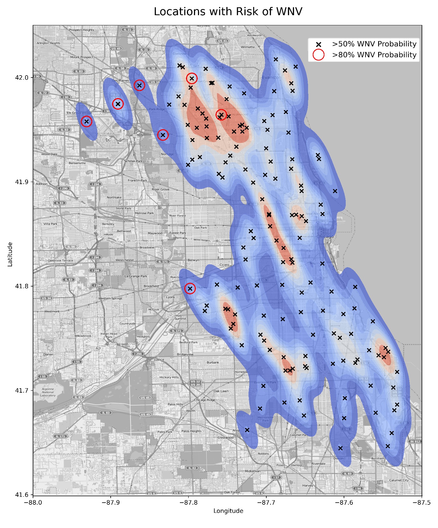
Recommendations¶

Our model has shown that certain areas are particularly 'dense' in terms of WNV-positive pools and pool proximity. In conjunction with this, our model also predicted several traps that have an 80% probability or greater of a WNV outbreak. We believe that the neighborhoods in which these traps are located should be an immediate focus for mosquito control efforts. These areas have been highlighted with a red circle below.

We've extrapolated that these are the neighborhoods that have a high risk of WNV:

Elk Grove Village (7,500 acres)
Des Plains (9,000 acres)
Norridge (1,100 acres)
Lincolnwood (1,700 acres)
Stickney (1,200 acres)
Forest View (900 acres)
Morton Grove (3,100 acres)

Around 24,500 acres of area in Chicago were identified as high risk, housing an approximate population of 148,500 people.

We recommend using the following methods to deal with areas with a high WNV risk:

Automation with drones

Drones can serve multiple purposes when it comes to combatting WNV:

They can collect aerial images that can be analyzed and used to identify and map breeding sites—such as cisterns, pots and buckets, old tires and flower pots. These images can be aggregated into accurate maps to support targeted application of larvicides (insecticides that specifically target the larval stage of an insect) at these potential breeding sites.
Once larval habitats are identified, drones can be equipped to carry and apply larvicides and/or adulticides to small targeted areas. These drones can also be fitted with a global positioning system (GPS) that can track flight patterns in conjunction with insecticide application. An operator can remotely pilot the drone or, in some cases, autopilot programs may be available for pre-programmed flights. Drones can be useful to target specific areas with larvicides or adulticides, as an alternative to truck-mounted applications that may require a high degree of drift of droplets to reach a target area in remote locations. These drones can spray potentially up to 80 acres in a day's work.

In summary, drones could be more environmentally friendly than doing the same spraying procedure on foot, and are likely to be a lot more accurate due to the ability to spray from a fully-vertical angle.

Adoption of best practices

The city of Chicago can aim to reduce spraying target areas by adopting guidelines from tropical countries like Singapore that have proven to be successful in combatting mosquito-borne viruses. For example, this could involve active on-the-ground checks of homes and premises for mosquito habitats, where public officers provide advice on steps you can take to prevent mosquito breeding and impose penalties if premises are found with mosquito breeding.

Through automation and more efficient mosquito vector control processes, we can reduce the cost of spraying, enabling the city of Chicago to save human lives and prevent further outbreaks of the West Nile Virus.

	Date	AvgSpeed	Cool	Depart	DewPoint	Heat	PrecipTotal	ResultDir	ResultSpeed	SeaLevel	StnPressure	Sunrise	Sunset	Tavg	Tmax	Tmin	WetBulb	lowvis	n_codesum	rain
0	2007-05-01	9.40	2.5	14.5	51.0	0.0	0.000	26.0	2.20	29.820	29.140	448.0	1849.0	67.5	83.5	51.0	56.5	0.0	0.0	0.0
1	2007-05-02	13.40	0.0	-2.5	42.0	13.5	0.000	3.0	13.15	30.085	29.410	447.0	1850.0	51.5	59.5	42.5	47.0	1.0	1.5	0.0
2	2007-05-03	12.55	0.0	3.0	40.0	8.0	0.000	6.5	12.30	30.120	29.425	446.0	1851.0	57.0	66.5	47.0	49.0	0.5	0.5	0.0
3	2007-05-04	10.60	0.0	7.0	41.5	4.0	0.005	7.5	10.25	30.045	29.335	444.0	1852.0	61.0	72.0	50.0	50.0	0.0	0.5	0.5
4	2007-05-05	11.75	0.0	5.0	38.5	5.0	0.010	7.0	11.45	30.095	29.430	443.0	1853.0	60.0	66.0	53.5	49.5	0.0	0.0	0.0

	Year	AvgTemp	JanDepart
0	2006	35.8	12.0
1	2007	27.9	4.1
2	2008	23.5	-0.3
3	2009	15.9	-7.9
4	2010	22.0	-1.8

	Year	AvgTemp	JulDepart
0	2006	76.5	2.5
1	2007	73.7	-0.3
2	2008	74.0	0.0
3	2009	69.4	-4.6
4	2010	77.7	3.7

	WeekAvgTemp	templag1	templag2	templag3	templag4
YearWeek
201440	57.142857	65.285714	62.142857	60.071429	74.428571
201441	53.714286	57.142857	65.285714	62.142857	60.071429
201442	54.000000	53.714286	57.142857	65.285714	62.142857
201443	54.642857	54.000000	53.714286	57.142857	65.285714
201444	50.200000	54.642857	54.000000	53.714286	57.142857

	model	train_auc	test_auc	precision	specificity	recall	f_score
0	gb	0.906145	0.840764	0.368421	0.995983	0.042424	0.076087
1	lr	0.852268	0.831593	0.636364	0.998661	0.042424	0.079545
2	ada	0.867175	0.830862	0.666667	0.998996	0.036364	0.068966
3	svc	0.854914	0.763826	0.000000	1.000000	0.000000	0.000000
4	rf	0.986407	0.761421	0.309091	0.974556	0.206061	0.247273
5	et	0.988624	0.704181	0.284483	0.972213	0.200000	0.234875
6	dt	0.988624	0.669090	0.260000	0.962839	0.236364	0.247619

	model	train_auc	test_auc	precision	specificity	recall	f_score
0	lr	0.858562	0.824015	0.136782	0.748577	0.721212	0.229952
5	ada	0.961739	0.810826	0.154657	0.838969	0.533333	0.239782
2	et	0.975888	0.810203	0.151877	0.833612	0.539394	0.237017
4	rf	0.991832	0.804253	0.180662	0.892200	0.430303	0.254480
6	gb	0.997989	0.799169	0.238095	0.951791	0.272727	0.254237
3	svc	0.940915	0.786723	0.146875	0.817208	0.569697	0.233540
1	dt	0.990348	0.741223	0.162857	0.901908	0.345455	0.221359

Logit Regression Results
Dep. Variable:	WnvPresent	No. Observations:	10506
Model:	Logit	Df Residuals:	10474
Method:	MLE	Df Model:	31
Date:	Mon, 28 Dec 2020	Pseudo R-squ.:	0.1758
Time:	16:40:50	Log-Likelihood:	-1780.9
converged:	True	LL-Null:	-2160.6
Covariance Type:	nonrobust	LLR p-value:	9.485e-140

	coef	std err	z	P>\|z\|	[0.025	0.975]
const	-4.3870	0.135	-32.457	0.000	-4.652	-4.122
WinterDepart	0.7603	0.112	6.810	0.000	0.541	0.979
templag3	0.1704	0.134	1.271	0.204	-0.092	0.433
templag2	-0.0126	0.127	-0.099	0.921	-0.262	0.236
Sunrise	0.7611	0.294	2.589	0.010	0.185	1.337
Week	0	nan	nan	nan	nan	nan
Species	0.4748	0.082	5.797	0.000	0.314	0.635
Month	0.6513	0.327	1.991	0.046	0.010	1.292
WeekPrecipTotal	0.4252	0.116	3.653	0.000	0.197	0.653
templag4	-0.0046	0.139	-0.033	0.974	-0.278	0.269
DewPoint	0	nan	nan	nan	nan	nan
WetBulb	0.0195	0.365	0.053	0.957	-0.697	0.736
Tmin	0.9364	0.412	2.273	0.023	0.129	1.744
Sunset	0.2117	0.428	0.495	0.620	-0.626	1.050
templag1	0.0064	0.100	0.064	0.949	-0.189	0.202
Tavg	0	nan	nan	nan	nan	nan
Longitude	-0.4973	0.087	-5.712	0.000	-0.668	-0.327
Cool	0.5244	0.390	1.346	0.178	-0.239	1.288
WeekAvgTemp	-0.0514	0.163	-0.316	0.752	-0.370	0.268
rainlag4	-0.2428	0.115	-2.111	0.035	-0.468	-0.017
Heat	0	nan	nan	nan	nan	nan
YearWeek	0.5375	0.090	5.981	0.000	0.361	0.714
Depart	-2.2908	0.467	-4.902	0.000	-3.207	-1.375
r_humid	0	nan	nan	nan	nan	nan
n_codesum	0.1024	0.140	0.731	0.465	-0.172	0.377
Tmax	1.3912	0.449	3.102	0.002	0.512	2.270
ResultSpeed	-0.0292	0.173	-0.169	0.866	-0.368	0.309
Trap_T900	0.0467	0.055	0.856	0.392	-0.060	0.154
rainlag1	0.0134	0.128	0.104	0.917	-0.238	0.265
Trap_T143	0.0703	0.030	2.378	0.017	0.012	0.128
humidlag2	-0.2872	0.110	-2.607	0.009	-0.503	-0.071
Trap_T003	0.1127	0.037	3.080	0.002	0.041	0.184
AvgSpeed	-0.0597	0.185	-0.322	0.747	-0.423	0.303
humidlag1	0.1649	0.112	1.471	0.141	-0.055	0.385
humidlag4	0.2462	0.091	2.709	0.007	0.068	0.424
Latitude	-0.1370	0.077	-1.787	0.074	-0.287	0.013
lowvis	-0.1691	0.132	-1.277	0.201	-0.428	0.090

	coefs	sm_coefs
templag2	-0.009	-0.013
ResultSpeed	-0.028	-0.029
WeekAvgTemp	-0.052	-0.051
AvgSpeed	-0.063	-0.060
Latitude	-0.138	-0.137
lowvis	-0.171	-0.169
rainlag4	-0.246	-0.243
humidlag2	-0.289	-0.287
Longitude	-0.498	-0.497
Depart	-2.302	-2.291

Battling THE WEST NILE VIRUS

Deciphering and re-engineering location, time and weather in the Windy City